N T Result
4 0 0.0
4 10 4.707364688019771E-6
4 20 1.3126420636755292E-5
5 0 0.0
5 10 3.267731327728599E-6
5 20 8.343575060356386E-6


PRISM is a probabilistic model checker, a tool for the modelling and analysis of systems which exhibit probabilistic behaviour. Probabilistic model checking is a formal verification technique. It is based on the construction of a precise mathematical model of a system which is to be analysed. Properties of this system are then expressed formally in temporal logic and automatically analysed against the constructed model.
PRISM has support for a wide range of probabilistic models:
In fact, PRISM's support for MDPs extends to the more general model of probabilistic automata (PAs) [Seg95], which does not require unique action names in each state. For background material on these models, look at the pointers to resources on the PRISM web site.
PRISM also supports non-probabilistic models, notably labelled transition systems (LTSs).
Models are supplied to the tool by writing descriptions in the PRISM language, a simple, high-level modelling language.
Properties of these models are written in the PRISM property specification language which is based on temporal logic. It incorporates several well-known probabilistic temporal logics:
The property language also supports costs and rewards, "numerical" properties, several other custom features and extensions, and also also incorporates the non-probabilistic temporal logics CTL (computation tree logic) and LTL.
PRISM performs probabilistic model checking, based on exhaustive search and numerical solution, to automatically analyse such properties. It also contains a discrete-event simulation engine for approximate model checking.
PRISM is known to run on Linux, Windows and macOS, both 64-bit and 32-bit versions.
You will need Java, version 11 or above. To run binary versions of PRISM, you only need the Java Runtime Environment (JRE), not the full Java Development Kit (JDK).
To compile PRISM from source, you need the Java Development Kit (JDK), GNU make and a C/C++ compiler (e.g. gcc/g++). For compilation under Windows, you will need Cygwin. See below for more information:
If you are installing on a completely fresh operating system installation (e.g. in a virtual machine), you may find the following scripts useful,
which install the required dependencies and PRISM itself. They can be found in the prism/etc/scripts directory:
If you don't yet have Java, install it, for example with the Temurin installer.
To install PRISM on Windows, just run the self-extracting installer which you downloaded. You do not need administrator privileges for this, just write-access to the directory chosen for installation.
If requested, the installer will place shortcuts to run PRISM on the desktop and/or start menu. If not, you can run by PRISM double-clicking the file xprism.bat (which may just appear as xprism) in the bin folder of your PRISM folder. If nothing happens, the most likely explanation is that Java is not installed or not in your path. To check, open a command prompt window, navigate to the PRISM directory, type cd bin, then xprism.bat and examine the resulting error. If you want to create shortcuts to xprism.bat manually, you will find some PRISM icons in the etc folder.
If you wish to use the command-line version of PRISM on Windows, open a command prompt window and type for example:
You can also edit the file bin\prism.bat to allow it to be run from any location. See the instructions within the file for further details.
Problems? See the section "Common Problems And Questions''.
We provide pre-compiled binary distributions for Linux and macOS
(if you have any problems running these, try compiling PRISM from source instead - see below for instructions).
To install a binary distribution, unpack the tarred/zipped PRISM distribution into a suitable location, enter the directory and run the install.sh script, e.g.:
On macOS, you may want to run the following command, which avoids manual approving the integrity of the binary files:
You do not need to be root to install PRISM. The install script simply makes some small customisations to the scripts used to launch PRISM. The PRISM distribution is self-contained and can be freely moved/renamed, however if you do so you will need to re-run ./install.sh afterwards.
To run PRISM, execute either the xprism or prism script (for the graphical user interface or command-line version, respectively). These can be found in the bin directory. These scripts are designed to be run from anywhere and you can easily create symbolic links or aliases to them. If you want icons to create desktop shortcuts to PRISM, you can find some in the etc directory.
Problems? See the section "Common Problems And Questions''.
To compile PRISM form source code, you will need:
To check that you have the development kit, type javac. If you get an error message that javac cannot be found, you probably do not have the JDK installed (or your path is not set up correctly). To check what version you have, type javac -version.
Hopefully, you can build PRISM simply by entering the PRISM directory and running make, e.g.:
For this process to complete correctly, PRISM needs to be able to determine your operating system (OSTYPE), machine architecture (ARCH) and the location of your Java distribution (JAVA_DIR). If there is a problem with either of these, you will see an error message and will need to specify one or more of these manually, such as in these examples:
Note the use of double quotes for the case where the directory contains a space. If you don't know the location of your Java installation, try typing which javac. If the result is e.g. /usr/java/jdk1.8.0/bin/javac then your Java directory is /usr/java/jdk1.8.0. Sometimes javac will be a symbolic link, in which case use "ls -l" to determine the actual location.
It is also possible to to set the environment variables directly or edit their values in the Makefile directly. Note that even when you specify JAVA_DIR explicitly (in either way), PRISM still uses the version of javac that is in your path. To override this, you can also specify a specific version by setting JAVAC.
Problems? See the section "Common Problems And Questions''.
The compilation of PRISM currently relies on a Unix-like environment. On Windows, this can be achieved using the Cygwin development environment, with the packages below installed. You can run the script prism-install-windows.bat in a Command Prompt to automate this.
make
mingw64-x86_64-gcc-g++ (for 64-bit Windows) or mingw64-i686-gcc-g++ (for 32-bit Windows)
binutils
dos2unix
git (if you will pull source code from GitHub)
wget (if you will pull source code from the web)
Then proceed as described in the previous section. Note that the PRISM compilation process uses the MinGW libraries so that the final result is independent of Cygwin at run-time.
One thing to note: make sure you unzip the PRISM distribution from within Cygwin (e.g. using tar xfz prism-XXX-src.tar.gz). Don't use a Windows program (Winzip, etc.) since this can cause problems.
If you use git to checkout the PRISM repository, we recommend that you use the version of git provided by Cygwin. If you use a native Windows version of git, you may want to disable the Unix-to-Windows line-ending conversion, e.g., via
git config --global core.autocrlf false
Problems? See the section "Common Problems And Questions''.
An alternative to Cygwin on Windows is MSYS2. You can install the required MSYS2 packages like this:
The environment is currently not directly supported in the Makefile, which can be fixed as follows:
Additionally, MSYS2 does not handle symlinks in the same way as Cygwin does.
At some point make will fail, saying that it cannot find the CUDD library.
You can solve this as follows:
Problems? See the section "Common Problems And Questions''.
This section describes some of the most common problems and questions related to the installation and running of PRISM. These are grouped into the following categories:
When I try to run PRISM on Windows, I double-click the PRISM shortcut but nothing happens.
The most common cause of this is that you either do not have Java installed or the java executable is not in your path. In any case, to determine the exact problem, launch a command shell and navigate to the bin directory inside the directory where you installed PRISM (you can use the "PRISM (console)" shortcut installed in the start menu to do this). Then, type prism.bat and see what error message is displayed.
When I try to run PRISM, I get one of these errors:
Exception in thread "main" java.lang.NoClassDefFoundError: ...
java.lang.UnsatisfiedLinkError: no prism in java.library.path
java.lang.UnsatisfiedLinkError: ...
Library not loaded: ../../lib/libdd.dylib
Things to check:
(1) Did you run install.sh from the PRISM directory? (non-Windows platforms)
(2) If you compiled PRISM from source code, are you sure no errors occurred during the process? To check, go into the PRISM directory, type make clean_all and then make, checking the output (especially at the end) carefully for any error messages.
(3) Are you running on Mac OS? See the next question.
(3) Are you running on an old version of Mac OS (notably El Capitan)? This had some issues with PRISM calling java.
A workaround is to specify the exact path to the java when running PRISM, e.g.:
PRISM_JAVA=/Library/Java/JavaVirtualMachines/jdk1.9.jdk/Contents/Home/bin/java prism
or by replacing the value of PRISM_JAVA directly in the prism script directly.
When I try to run PRISM on macOS, I get an error of the form: "libprism.dylib can�t be opened because Apple cannot check it for malicious software." or "libprism.dylib not valid for use in process: library load disallowed by system policy".
PRISM's macOS binaries are currently not signed/notarised,
so you need to approve the binary files manually to run them.
Run this command from the same place you ran ./install.sh:
or approve the libraries one by one through the security settings.
You can also avoid this issue by compiling from source code.
When I try to run PRISM, I get an error of the form:Exception in thread "main" java.lang.UnsupportedClassVersionError: Bad version number in .class file
Your version of Java is too old. Update or install a newer version of Java, and then try again.
When I try to compile PRISM, make seems to get stuck in an infinite loop
This is probably due to the detection of Java failing. Specify the location of your Java directory by hand, e.g. make JAVA_DIR=/usr/java/jdk1.9.0. See the Instructions page for more on this.
When I try to compile PRISM, I get errors of the form:/usr/bin/libtool: for architecture: cputype (16777234) cpusubtype (0) file: -lSystem is not an object file (not allowed in a library)
Are you compiling PRISM on Max OS X? If so, the likely explanation is that you have upgraded to a new version of Mac OS X but have not upgraded the developer tools (eg. XCode). Upgrade and try again.
When I try to compile PRISM, nothing seems to happen
Perhaps you are not using the GNU version of make. Try typing make -v to find out. On some systems, GNU make is called gmake.
When I try to compile PRISM, I get errors of the form:Unexpected end of line seen...
or:make: Fatal error in reader: Makefile, line 58: Unexpected end of line seen...
Perhaps you are not using the GNU version of make. Try typing make -v to find out. On some systems, GNU make is called gmake.
When I try to compile PRISM, I get an error of the form:./setup.sh: line 33: syntax error: unexpected end of file
Are you building on Cygwin? And did you unpack PRISM using WinZip? If so, unpack from Cygwin, using tar xfz (or similar) instead.
When I try to compile PRISM, I get an error of the form:Assembler messages: Fatal error: can't create ../../obj/dd/dd_abstr.o: No such file or directory
Did you unpack PRISM using a graphical tool or file manager? If so, unpack using tar xfz (or similar) instead.
Do I have to use GNU make to build PRISM?
Strictly speaking, no, but you will have to modify the various PRISM Makefiles manually to overcome this.
Can I build PRISM on operating systems other than those currently supported?
PRISM should be suitable for any Unix/Linux variant.
The first thing you will need to do is compile CUDD (the BDD library used by and included in PRISM) on that platform.
Fortunately, CUDD has already been successfully built on a large number of
operating systems. Have a look at the sample Makefiles we provide (i.e. the
files cudd/Makefile.*) which are slight variants of the original Makefile
provided with CUDD (found here: cudd/modified/orig/Makefile). They contain
instructions on how to modify it for various platforms. You can then call
your new modified makefile something appropriate (cudd/Makefile.$OSTYPE) and
proceed to build PRISM as usual. To just build CUDD, not PRISM, type
make cuddpackage instead of make.
Next, look at the main PRISM Makefile, in particular, each place where the
variable $OSTYPE is referred to. Most lines include comments and further
instructions. Once you have done this, proceed as usual.
If you do successfully build PRISM on other platforms, please let us know so we can include this information in future releases. Thanks.
How do I uninstall PRISM?
If you installed PRISM on Windows using the self-extracting installer, you can uninstall it using the option on the start menu. If you didn't add these shortcuts, just run uninstall.exe from the directory where you installed PRISM.
For older versions of PRISM on Windows or on any other platform, simply delete the directory containing it.
The only thing that is not removed via either of these methods is the .prism file containing your PRISM settings which is in your home directory (see the section "Configuring PRISM"). You may wish to retain this when upgrading.
I still have a problem installing/running PRISM. What can I do?
Please post a message in the discussion group (see the support section of the PRISM website).
In order to construct and analyse a model with PRISM, it must be specified in the PRISM language, a simple, state-based language, based on the Reactive Modules formalism of Alur and Henzinger [AH99]. This is used for all of the types of model that PRISM supports.
In this section, we describe the PRISM language and present a number of small illustrative examples.
A precise definition of the semantics of the language is available from the "Documentation" section of the PRISM web site. One of the best ways to learn what can be done with the PRISM language is to look at some existing examples.
A number of these are included with the tool distribution in the prism-examples directory.
Many additional examples can be found on the "Case Studies" section of the PRISM website.
The fundamental components of the PRISM language are modules and variables. A model is composed of a number of modules which can interact with each other. A module contains a number of local variables. The values of these variables at any given time constitute the state of the module. The global state of the whole model is determined by the local state of all modules. The behaviour of each module is described by a set of commands. A command takes the form:
The guard is a predicate over all the variables in the model (including those belonging to other modules). Each update describes a transition which the module can make if the guard is true. A transition is specified by giving the new values of the variables in the module, possibly as a function of other variables. Each update is assigned a probability (or in some cases a rate) which will be assigned to the corresponding transition. The command also optionally includes an action, either just to annotate it, or for synchronisation.
We will use the following simple example to illustrate the basic concepts of the PRISM language. Consider a system comprising two identical processes which must operate under mutual exclusion. Each process can be in one of 3 states: {0,1,2}. From state 0, a process will move to state 1 with probability 0.2 and remain in the same state with probability 0.8. From state 1, it tries to move to the critical section: state 2. This can only occur if the other process is not in its critical section. Finally, from state 2, a process will either remain there or move back to state 0 with equal probability. The PRISM code to describe an MDP model of this system can be seen below. In the next sections, we explain each aspect of the code in turn.
The PRISM Language: Example 1
As mentioned above, the PRISM language can be used to describe several types of probabilistic models. To indicate which type is being described, a PRISM model usually includes a model type keyword:
dtmc: discrete-time Markov chain
ctmc: continuous-time Markov chain
mdp: Markov decision process (or probabilistic automaton)
pta: probabilistic timed automaton
pomdp: partially observable Markov decision process
popta: partially observable probabilistic timed automaton
This is typically at the very start of the file, but can actually occur anywhere in the file (except inside modules and other declarations).
If no such model type declaration is included, the model is by default assumed to be an MDP. PRISM also performs some auto-detection of the model type; for example, an MDP with clock variables is assumed to be a PTA, and an MDP with observables? is assumed to be a POMDP.
Note: For compatibility with old versions of PRISM,
the keywords probabilistic, stochastic and nondeterministic
can be used as alternatives for dtmc, ctmc and mdp, respectively.
The previous example uses two modules, M1 and M2, one representing each process.
A module is specified as:
The definition of a module contains two parts: its variables and its commands. The variables describe the possible states that the module can be in; the commands describe its behaviour, i.e. the way in which the state changes over time. Currently, PRISM supports just a few simple types of variables: they can either be (finite ranges of) integers or Booleans (we ignore clocks for now).
In the example above, each module has one integer variable with range [0..2].
A variable declaration looks like:
Notice that the initial value of the variable is also specified. A Boolean variable is declared as follows:
It is also possible to omit the initial value of a variable,
in which case it is assumed to be the lowest value in the range (or false for a Boolean).
Thus, the variable declarations shown below are equivalent to the ones above.
As will be described later, it is also possible to specify
multiple initial states for a model.
We also mention that, for a few kinds of model analysis (typically those based on simulation, such as approximate model checking or fast adaptive simulation, it is also permissable to use integer variables with unbounded ranges, denoted as:
Where the state space of the model remains finite, despite the presence of such unbounded variables, you can use the explicit engine to build and analyse the model.
The names given to modules and variables are referred to as identifiers.
Identifiers can be made up of letters, digits and the underscore character, but cannot begin with a digit,
i.e. they must satisfy the regular expression [A-Za-z_][A-Za-z0-9_]*, and are case-sensitive.
Furthermore, identifiers cannot be any of the following, which are all reserved keywords in PRISM:
A,
bool,
clock,
const,
ctmc,
C,
double,
dtmc,
E,
endinit,
endinvariant,
endmodule,
endobservables,
endrewards,
endsystem,
false,
formula,
filter,
func,
F,
global,
G,
init,
invariant,
I,
int,
label,
max,
mdp,
min,
module,
X,
nondeterministic,
observable,
observables,
of,
Pmax,
Pmin,
P,
pomdp,
popta,
probabilistic,
prob,
pta,
rate,
rewards,
Rmax,
Rmin,
R,
S,
stochastic,
system,
true,
U,
W.
The behaviour of each module is described by commands,
comprising a guard and one or more updates.
The first command of module M1 in our example is:
The guard x=0 indicates that this describes the behaviour of the module when the variable x has value 0.
The updates (x'=0) and (x'=1) and their associated probabilities state that the value of x will
remain at 0 with probability 0.8 and change to 1 with probability 0.2.
Note that the inclusion of updates in parentheses, e.g. (x'=1), is essential.
While older versions of PRISM did not report the absence of parentheses as an error, newer versions do.
Note also that PRISM will complain if the probabilities on the right hand side of a command do not sum to one.
The second command:
illustrates that guards can contain constraints on any variable, not just the ones in that module,
i.e. the behaviour of one module can depend on the state of another.
Updates, however, can only specify values for variables belonging to the module.
In general a module can read the variables of any other module, but only write to its own.
When a command comprises a single update with probability 1, the 1.0: can be omitted,
as is done in the example above.
If a module has more than one variable, updates describe the new value for each of them.
For example, if it had two variables x1 and x2, a possible command would be:
Notice that elements of the updates are concatenated with & and that each element must be bracketed individually.
If an update does not give a new value for a local variable, it is assumed not to change.
As a special case, the keyword true can be used to denote an update where no variable's value changes, i.e. the following are all equivalent:
Finally, it is important to remember that the expressions on the right hand side of each update refer to the state of the model before the update occurs. So, for example, this command:
updates variable x2 to 0, not 2.
The probabilistic model corresponding to a PRISM language description is constructed as the parallel composition of its modules. In every state of the model, there is a set of commands (belonging to any of the modules) which are enabled, i.e. whose guards are satisfied in that state. The choice between which command is performed (i.e. the scheduling) depends on the model type.
For an MDP, as in Example 1, the choice is nondeterministic. By way of example, consider state (0,0) (i.e. x=0 and y=0). There are two commands enabled, one from each module:
In state (0,0) of the MDP, there would be a nondeterministic choice between these two probability distributions:
0.8:(0,0) + 0.2:(1,0) (module M1 moves)
0.8:(0,0) + 0.2:(0,1) (module M2 moves)
For a DTMC, the choice is probabilistic: each enabled command is selected with equal probability.
If Example 1 was a DTMC, then in state (0,0) of the model
the following probability distribution would result:
0.8:(0,0) + 0.1:(1,0) + 0.1:(0,1)
For a CTMC, as will be discussed shortly, the choice is modelled as a "race" between transitions.
See the later sections on "Synchronisation" and "Process Algebra Operators" for other topics related to parallel composition.
PRISM models that support nondeterminism, such as are MDPs, can also exhibit local nondeterminism,
which allows the modules themselves to make nondeterministic choices.
In Example 1, we can make the probabilistic choice in the first state of module M1 nondeterministic by replacing the command:
with the commands:
Assuming we do the same for module M2, in state (0,0) of the MDP
there will be a nondeterministic choice between the three (trivial) probability distributions listed below. (There are three, not four, distributions because two possibilities result in identical behaviour: staying with probability 1 in the state state.)
1.0:(0,0)
1.0:(1,0)
1.0:(0,1)
More generally, local nondeterminism can also arise when the guards of two commands overlap only partially, rather than completely as in the example above.
PRISM also permits local nondeterminism in models which are DTMCs, although the nondeterministic choice is randomised when the parallel composition of the modules occurs. Since the appearance of nondeterminism in a DTMC is often the result of a user error in the model specification, PRISM displays a warning when local nondeterminism is detected in a DTMC. Overlapping guards in CTMCs are not treated as nondeterministic choices.
Specifying the behaviour of a continuous-time Markov chain (CTMC) is done in similar fashion to a DTMC or an MDP, as discussed so far. The main difference is that updates in commands are labelled with (positive-valued) rates, rather than probabilities. The notation used in commands, however, to associate rates to transitions is identical to the one used to assign probabilities:
In a CTMC, when multiple possible transitions are available in a state, a race condition occurs (see e.g. [KNP07a] for more details). In terms of PRISM commands, this can arise in several ways. Firstly, within in a module, multiple transitions can be specified either as several different updates in a command, or as multiple commands with overlapping guards. The following, for example. are equivalent:
Furthermore, parallel composition between modules in a CTMC is modelled as a race condition, rather as a nondeterministic choice, like for MDPs.
We now introduce a second example: a CTMC that models an N-place queue of jobs and a server which removes jobs from the queue and processes them. The PRISM code is as follows:
The PRISM Language: Example 2
This example also introduces a number of other PRISM language concepts, including constants, action labels and synchronisation. These are described in the following sections.
PRISM supports the use of constants, as seen in Example 2.
Constants can be integers, doubles or Booleans
and can be defined using literal values or as constant expressions (including in terms of each other) using the const
keyword. For example:
The identifiers used for their names are subject to the same rules as variables.
Constants can be used anywhere that a constant value would be expected,
such as the lower or upper range of a variable (e.g. N in Example 2),
the probability or rate associated with an update (mu in Example 2),
or anywhere in a guard or update.
As will be described later constants can also be left undefined
and specified later, either to a single value or a range of values, using experiments.
Note: For the sake of backward-compatibility, the notation used in earlier versions of PRISM
(const for const int and rate or prob for const double) is still supported.
The definition of the area constant, in the example above, uses an expression.
We now define more precisely what types of expression are supported by PRISM.
Expressions can contain literal values (12, 3.141592, true, false, etc.),
identifiers (corresponding to variables, constants, etc.) and operators from the following list:
- (unary minus)
^ (power)
*, / (multiplication, division)
+, - (addition, subtraction)
<, <=, >=, > (relational operators)
=, != (equality operators)
! (negation)
& (conjunction)
| (disjunction)
<=> (if-and-only-if)
=> (implication)
? (condition evaluation: condition ? a : b means "if condition is true then a else b")
All of these operators except ? and => are left associative
(i.e. they are evaluated from left to right).
The precedence of the operators is as found in the list above,
most strongly binding operators first.
Operators on the same line (e.g. + and -) are of equal precedence.
Much of the notation for expressions is hence essentially equivalent to that of C/C++ or Java.
One notable exception to this is that the division operator / always performs floating point, not integer, division,
i.e. the result of 22/7 is 3.142857... not 3.
All expressions must evaluate correctly in terms of type (integer, double or Boolean).
Built-in Functions
Expressions can make use of several built-in functions:
min(...) and max(...), which select the minimum and maximum value, respectively, of two or more numbers
floor(x) and ceil(x), which round x down and up, respectively, to the nearest integer
round(x), which rounds x to the nearest integer (note, in a tie-break, we always round up, e.g. round(-1.5) gives -1 not -2)
pow(x,y) which computes x to the power of y (same as x^y)
mod(i,n) for integer modulo operations
log(x,b), which computes the logarithm of x to base b
Examples of their usage are:
For compatibility with older versions of PRISM, all functions can also be expressed via the func keyword, e.g. func(floor, 13.5).
Use of Expressions
Expressions can be used in a wide range of places in a PRISM language description, e.g.:
This allows, for example, the probability in a command to be dependent on the current state:
Another feature of PRISM introduced in Example 2 is synchronisation.
In the style of many process algebras, we allow commands to be labelled with actions.
These are placed inside the square brackets which mark the start of the command,
for example serve in this command from Example 2:
These actions can be used to force two or more modules to make transitions simultaneously
(i.e. to synchronise).
For example, in state (3,0) (i.e. q=3 and s=0),
the composed model can move to state (2,1),
synchronising over the serve action.
The rate of this transition is equal to the product of the two individual rates
(in this case, lambda * 1 = lambda).
The product of two rates does not always meaningfully represent the rate of a synchronised transition.
A common technique, as seen here, is to make one action passive, with rate 1 and one action active,
which actually defines the rate for the synchronised transition.
By default, all modules are combined using the standard CSP parallel composition
(i.e. modules synchronise over all their common actions).
PRISM also supports module renaming, which allows duplication of modules.
In Example 1, module M2 is identical to module M1 so we can in fact replace its entire definition with:
All of the variables in the module being renamed (in this case, just x) must be renamed to new, unused names. Optionally, it is also possible to rename other aspects of the module definition. In fact, the renaming is done at a textual level, so any identifiers (including action labels, constants and functions) used in the module definition can be changed in this way.
Note: Care should be taken when renaming modules that make use of formulas.
Typically, a variable declaration
specifies the initial value for that variable.
The initial state for the model is then defined by the initial value for all variables.
It is possible, however, to specify that a model has multiple initial states.
This is done using the init...endinit construct,
which can be placed anywhere in the file except within a module definition,
and removing any initial values from variable declarations.
Between the init and endinit keywords, there should be a
predicate over all the variables of the model.
Any state which satisfies this predicate is an initial state.
Consider again Example 1.
As it stands, there is a single initial state (0,0) (i.e. x=0 and y=0).
If we remove the init 0 part of both variable declarations
and add the following to the end of the file:
there will be three initial states: (0,0), (0,1) and (0,2).
Similarly, we could instead add:
in which case there would be two initial states: (0,1) and (1,0).
In addition to the local variables belonging to each module, a PRISM model can also include global variables, which can be written to, as well as read, by all modules. Like local variables, these can be integers or Booleans. Global variables are declared in identical fashion to a module's local variables, except that the declaration must not be inside the definition of any module. Some example declarations are as follows:
A global variable can be modified by any module and provides another way for modules to interact. An important restriction on the use of global variables is the fact that commands which synchronise with other modules (i.e. those with an action label attached; see the section "Synchronisation") cannot modify global variables. PRISM will detect this and report an error.
PRISM models can include formulas which are used to avoid duplication of code. A formula comprises a name (an identifier) and an expression. The formula name can then be used as shorthand for the expression anywhere an expression might usually be accepted. A formula is defined as follows:
It can then be used anywhere within that file, as for example in this command:
The effect is exactly as if the following had been typed:
Formulas defined in a model can also be used when specifying its properties.
During parsing of the model, expansion of formulas is done before module renaming so, if a module which uses formulas is renamed to another module, it is the contents of the formula which will be renamed, not the formula itself.
PRISM models can also contain labels. These are a way of identifying sets of states that are of particular interest. Labels can only be used when specifying properties but, for convenience, can be defined in model files as well as property files.
Labels differ from formulas in two other ways: firstly, they must be of Boolean type;
secondly, they are written using quotation marks ("..."), as illustrated in the following example:
PRISM supports the specification and analysis of properties based on costs and rewards. This means that it can be used to reason, not just about the probability that a model behaves in a certain fashion, but about a wider range of quantitative measures relating to model behaviour. For example, PRISM can be used to compute properties such as "expected time", "expected number of lost messages" or "expected power consumption". The implementation of cost- and reward-based techniques in the tool is only partially completed and is still ongoing. If you have questions, comments or feature-requests relating to this functionality, please feel free to contact the PRISM team about this.
The basic idea is that probabilistic models (of all types) developed in PRISM can be augmented with costs or rewards: real values associated with certain states or transitions of the model. In fact, since there is no practical distinction between costs and rewards (except that costs are generally perceived to be "bad" and rewards to be "good"), PRISM only supports rewards. The user is, however, free to interpret the values however they choose.
In this section, we describe how models described in the PRISM language
can be augmented with rewards.
Later, we will discuss how to express properties that relate to these rewards.
Rewards are associated with models using rewards ... endrewards constructs,
which can appear anywhere in a model file except within a module definition.
These constructs contains one or more reward items.
Consider the following simple example:
This defines a reward structure with name r1 (the name is optional)
which assigns a reward of 1 to every state of the model.
It comprises a single reward item, the left part of which (true) is a guard
and the right part of which (1) is a reward.
States of the model which satisfy the predicate in the guard are assigned the corresponding reward.
More generally, state rewards can be specified using multiple reward items,
each of the form guard : reward;,
where guard is a predicate (over all the variables of the model)
and reward is an expression (containing any variables, constants, etc. from the model).
For example:
assigns a reward of 100 to states satisfying x=0 or x=10
and a reward of 2*x to states satisfying x>0 & x<10.
Note that a single reward item can assign different rewards to different states,
depending on the values of model variables in each one.
Any states which do not satisfy the guard of any reward item will have no reward assigned to them.
For states which satisfy multiple guards, the reward assigned to the state
is the sum of the rewards for all the corresponding reward items.
Rewards can also be assigned to transitions of a model.
These are specified in a similar fashion to state rewards,
within the rewards ... endrewards construct.
Reward items describing transition rewards are of the form [action] guard : reward;,
the interpretation being that transitions from states which satisfy the guard guard
and are labelled with the action action acquire the reward reward.
For example:
assigns a reward of 1 to all transitions in the model with no action label,
and rewards of x and 2*x to all transitions labelled with actions a and b, respectively.
As is the case for states, multiple reward items can specify rewards for a single transition,
in which case the resulting reward is the sum of all the individual rewards.
A model description can specify rewards for both states and transitions.
These are all placed together in a single rewards...endrewards construct.
A PRISM model will often have multiple reward structures, for example:
So far in this section, we have mainly focused on three types of models: DTMCs, MDPs and CTMCs,
in which all the variables making up their state are finite.
PRISM also supports real-time models, in particular,
probabilistic timed automata (PTAs), which extend MDPs with the ability to model real-time behaviour.
This is done in the style of timed automata [AD94], by adding clocks,
real-valued variables which increase with time and can be reset. For background material on PTAs, see for example [NPS13].
You can also find several example PTA models included in the PRISM distribution. Look in the prism-examples/ptas directory.
Before describing how PTA features are incorporated into the PRISM modelling language, we give a simple example. Here is a small PTA:
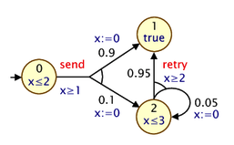
and here is a corresponding PRISM model:
For modelling PTAs in PRISM, there is a new datatype, clock, used for variables that are clocks. Other types of PRISM variables can be defined in the usual way. In the example above, we use just a single integer variable s to represent the locations of the PTAs.
In a PTA, transitions can include a guard, which constrains when it can occur based on the current value of clocks, and resets, which specify that a clock's values should be set to a new (integer) value. These are both specified in PRISM commands in the usual way: see, for example, the inclusion of x>=1 in the guard for the send-labelled command and the updates of the form (x'=0) which reset the clock x to 0.
The other new addition is an invariant construct, which is used to specify an expression describing the clock invariants for each PRISM module. These impose restrictions on the allowable values of clock variables, depending on the values of the other non-clock variables. The invariant construct should appear between the variable declarations and the commands of the module. Often, clock invariants are described separately for each PTA location; hence, the invariant will often take the form of a conjunction of implications, as in the example model above, but more general expressions are also permitted. In the example, the clock x must satisfy x<=2 or x<=3 when local variables s is 0 or 2, respectively. If s is 1, there is no restriction (since the invariant is effectively true in this case).
Expressions that include reference to clocks, whether in guards or invariants, must satisfy certain conditions to facilitate model checking. In particular, references to clocks must appear as conjunctions of simple clock constraints, i.e. conjunctions of expressions of the form x~c or x~y where x and y are clocks, c is an integer-valued expression and ~ is one of <, <=, >=, >, =).
There are also some additional restrictions imposed on PTA models that are dependent on which of the PTA model checking engines is in use.
For the stochastic games and backwards reachability engines:
init...endinit construct is not permitted).
For the digital clocks engine:
x<=5 is allowed, but x<5 is not.
x<=y.
Finally, PRISM makes several assumptions about PTAs, regardless of the engine used.
PRISM supports analysis of partially observable probabilistic models,
most notably partially observable Markov decision processes (POMDPs),
but also partially observable probabilistic timed automata (POPTAs).
POMDPs are a variant of MDPs in which the strategy/policy
which resolves nondeterministic choices in the model is unable to
see the precise state of the model, but instead just observations of it.
For background material on POMDPs and POPTAs, see for example [NPZ17].
You can also find several example models included in the PRISM distribution.
Look in the prism-examples/pomdps and prism-examples/poptas directories.
PRISM currently supports state-based observations: this means that, upon entering a new POMDP state, the observation is determined by that state. In the same way that a model state comprises the values or one or more variables, an observation comprises one or more observables. There are several way to define these observables. The simplest is to specify a subset of the model's variables that are designated as being observable. The rest are unobservable.
For example, in a POMDP with 3 variables, s, l and h, the following:
specifies that s and l are observable and h is not.
Alternatively, observables can be specified as arbitrary expressions over variables.
For example, assuming the same variables s, l and h, this specification:
defines 2 observables. The first is, as above, the variable s.
The second, named "pos", determines if variable l is positive.
Other than this, the values of l and h are unobservable.
The named observables can then be used in properties
in the same way that labels can.
The above two styles of definition can also be mixed to specify a combined set of observables.
POPTAs (partially observable PTAs) combine the features of both PTAs and POMDPs. They are are currently analysed using the digital clocks engine, so inherit the restrictions for that engine. Furthermore, for a POPTA, all clock variables must be observable.
PRISM has support for uncertain models, in which there is epistemic uncertainty regarding some quantitative aspects of the probabilistic models being verified. In particular, it currently supports interval MDPs (IMDPs) and interval DTMCs (IDTMCs), which are MDPs or DTMCs in which transition probabilities can be specified as intervals, indicating that the exact probability is not precisely known. This can be useful, for example, when the transition probabilities have been estimated from data.
Currently, this is achieved by simply replacing the probabilities attached to updates in commands with intervals, e.g.:
As usual, the probability thresholds can be expressions involving state variables or constants, for example:
When two commands in different modules synchronise and specify the probabilities for updates to variables as intervals, these are considered to be independent, i.e., the probability of each combined transition is taken to be the product of the two component intervals.
See the property specification section for details of how these models are analysed.
To make the concept of synchronisation described above more powerful,
PRISM allows you to define precisely the way in which the set of modules are composed in parallel.
This is specified using the system ... endsystem construct,
placed at the end of the model description, which should contain a process-algebraic expression.
This expression should feature each module exactly once, and can use the following (CSP-based) operators:
M1 || M2 : alphabetised parallel composition of modules M1 and M2 (synchronising on only actions appearing in both M1 and M2)
M1 ||| M2 : asynchronous parallel composition of M1 and M2 (fully interleaved, no synchronisation)
M1 |[a,b,...]| M2 : restricted parallel composition of modules M1 and M2 (synchronising only on actions from the set {a, b,...})
M / {a,b,...} : hiding of actions {a, b, ...} in module M
M {a<-b,c<-d,...} : renaming of actions a to b, c to d, etc. in module M.
The first two types of parallel composition (|| and |||) are associative and can be applied to more than two modules at once.
When evaluating the expression, the hiding and renaming operators bind more tightly than the three parallel composition operators.
No other rules of precedence are defined and parentheses should be used to specify the order in which modules are composed.
Some examples of expressions which could be included in the system ... endsystem construct are as follows:
(station1 ||| station2 ||| station3) |[serve]| server
((P1 |[a]| P2) / {a}) || Q
((P1 |[a]| P2) {a<-b}) |[b]| Q
When no parallel composition is specified by the user,
PRISM implicitly assumes an expression of the form M1 || M2 || ... containing all of the modules in the model.
For a more formal definition of the process algebra operators described above, check the semantics of the PRISM language, available from the "Documentation" section of the PRISM web site.
PRISM is also able to import model descriptions written in (a subset of) the stochastic process algebra PEPA [Hil96].
Files containing model descriptions written in the PRISM language
can contain any amount of white space (spaces, tabs, new lines, etc.),
all of which is ignored when the file is parsed by the tool.
Comments can also be used included in files in the style of the C programming language,
by preceding them with the characters //.
This is illustrated by the PRISM language examples from earlier in this section.
We recommend that the .prism extension is used for PRISM model files.
Historically (when the tool supported fewer types of model),
different extensions were often used for each model type:
.nm for MDPs or PTAs, .pm for DTMCs and .sm for CTMCs.
In order to analyse a probabilistic model which has been specified and constructed in PRISM, it is necessary to identify one or more properties of the model which can be evaluated by the tool. PRISM's property specification language subsumes several well-known probabilistic temporal logics, including PCTL, CSL, probabilistic LTL and PCTL*. PCTL is used for specifying properties of discrete-time models such as DTMCs or PTAs, and also real-time models such as PTAs; CSL is an extension of PCTL for CTMCs; LTL and PCTL* can be used to specify properties of discrete-time models (or untimed properties of CTMCs). PRISM also supports most of the (non-probabilistic) temporal logic CTL.
In fact, PRISM also supports numerous additional customisations and extensions of these two logics. Full details of the property specifications permitted in PRISM are provided in the following sections. The presentation given here is relatively informal. For the precise syntax and semantics of the various logics, see [HJ94],[BdA95] for PCTL, [ASSB96],[BKH99] for CSL and, for example, [Bai98] for LTL and PCTL*. You can also find various pointers to useful papers in the About and Documentation sections of the PRISM website.
Before discussing property specifications in more detail, it is perhaps instructive to first illustrate some typical examples of properties which PRISM can handle. The following are a selection of such properties. In each case, we give both the PRISM syntax and a natural language translation:
"the algorithm eventually terminates successfully with probability 1"
"the probability that more than 5 errors occur within the first 100 time units is less than 0.1"
"in the long-run, the probability that an inadequate number of sensors are operational is less than 0.01"
Note that the above properties are all assertions, i.e. ones to which we would expect a "yes" or "no" answer. This is because all references to probabilities are associated with an upper or lower bound which can be checked to be either true or false. In PRISM, we can also directly specify properties which evaluate to a numerical value, e.g.:
"the probability that process 1 terminates before process 2 does"
"the maximum probability that more than 10 messages have been lost by time T" (for an MDP/PTA)
"the long-run probability that the queue is more than 75% full"
Furthermore, PRISM makes it easy to combine such properties into more complex expressions, compute their values for a range of parameters and plot graphs of the results using experiments. This is often a very useful way of identifying interesting patterns or trends in the behaviour of a system. See the Case Studies section of the PRISM website for many examples of this kind of analysis.
One of the most fundamental tasks when specifying properties of a model is to identify particular sets or classes of states of the model. For example, to verify a property such as "the algorithm eventually terminates successfully with probability 1", it is first necessary to identify the states of the model which correspond to situations where "the algorithm has terminated successfully". In terms of the way temporal logics are usually presented, these correspond to atomic propositions.
In PRISM, this is achieved simply by writing an expression in the PRISM language which evaluates to a Boolean value. This expression will typically contain references to variables (and constants) from the model to which it relates. The set of states corresponding to this expression is those for which it evaluates to true. We say that the expression is "satisfied" in these states.
For example, in the property given above:
the expression num_errors > 5 is used to identify states of the model where more than 5 errors have occurred.
It is also common to use labels to identify states in this way, like "terminate" in the example:
Properties can refer to labels either from the model to which the property relates, or included in the same properties file.
One of the most important operators in the PRISM property specification language is the P operator, which is used to reason about the probability of an event's occurrence. This operator was originally proposed in the logic PCTL but also features in the other logics supported by PRISM, such as CSL. The P operator is applicable to all types of models supported by PRISM.
Informally, the property:
is true in a state s of a model if
"the probability that path property pathprop is satisfied by the paths from state s
meets the bound bound".
A typical example of a bound would be:
which means: "the probability that pathprop is satisfied by the paths from state s is greater than 0.98". More precisely, bound can be any of >=p, >p, <=p or <p,
where p is a PRISM language expression evaluating to a double in the range [0,1].
The types of path property supported by PRISM and their semantics will be discussed shortly.
For models that can exhibit nondeterministic behaviour, such as MDPs or PTAs, some additional clarifications are necessary. Whereas for fully probabilistic models such as DTMCs and CTMCs, probability measures over paths are well defined (see e.g. [KSK76] and [BKH99], respectively), for nondeterministic models a probability measure can only be feasibly defined once all nondeterminism has been removed.
Hence, the actual meaning of the property P bound [ pathprop ] in these cases is:
"the probability that pathprop is satisfied by the paths from state s
meets the bound bound for all possible resolutions of nondeterminism".
This means that, properties using the P operator then effectively reason about the
minimum or maximum probability, over all possible resolutions of nondeterminism,
that a certain type of behaviour is observed.
This depends on the bound attached to the P operator:
a lower bound (> or >=) relates to minimum probabilities
and an upper bound (< or <=) to maximum probabilities.
It is also very often useful to take a quantitative approach to probabilistic model checking, computing the actual probability that some behaviour of a model is observed,
rather than just verifying whether or not the probability is above or below a given bound.
Hence, PRISM allows the P operator to take the following form:
These properties return a numerical rather than a Boolean value. The S and R operators, discussed later, can also be used in this way.
As mentioned above, for nondeterministic models (MDPs or PTAs), either minimum or maximum probability values can be computed. Therefore, in this case, we have two possible types of property:
which return the minimum and maximum probabilities, respectively.
It is also possible to specify to which state the probability returned by a quantitative property refers. This is covered in the later section on filters.
PRISM supports a wide range of path properties that can be used with the P operator.
A path property is a formula that evaluates to either true or false for a single path in a model.
Here, we review some of the simpler properties that feature a single temporal operator,
as used for example in the logics PCTL and CSL. Later, we briefly describe how PRISM also supports more complex LTL-style path properties.
The basic different types of path property that can be used inside the P operator are:
X : "next"
U : "until"
F : "eventually" (sometimes called "future")
G : "always" (sometimes called "globally")
W : "weak until"
R : "release"
In the following sections, we describe each of these temporal operators. We then discuss the (optional) use of time bounds with these operators. Finally, we also discuss LTL-style path properties.
The property X prop is true for a path if prop is true in its second state,
An example of this type of property, used inside a P operator, is:
which is true in a state if "the probability of the expression y=1 being true in the next state is less than 0.01".
The property prop1 U prop2 is true for a path if
prop2 is true in some state of the path and prop1 is true in all preceding states.
A simple example of this would be:
which is true in a state if "the probability that z is eventually equal to 2, and that z remains less than 2 up until that point, is greater than 0.5".
The property F prop is true for a path if prop eventually becomes true at some point along the path. The F operator is in fact a special case of the U operator (you will often see F prop written as true U prop). A simple example is:
which is true in a state if "the probability that z is eventually greater than 2is less than 0.1".
Whereas the F operator is used for "reachability" properties, G represents "invariance". The property G prop is true of a path if prop remains true at all states along the path. Thus, for example:
states that, with probability at least 0.99, z never exceeds 10.
Like F and G, the operators W and R are derivable from other temporal operators.
Weak until (a W b), which is equivalent to (a U b) | G a, requires that a remains true until b becomes true, but does not require that b ever does becomes true (i.e. a remains true forever). For example, a weak form of the until example used above is:
which states that, with probability greater than 0.5, either z is always less than 2, or it is less than 2 until the point where z is 2.
Release (a R b), which is equivalent to !(!a U !b), informally means that b is true until a becomes true, or b is true forever.
All of the temporal operators given above, with the exception of X, have "bounded" variants, where an additional time bound is imposed on the property being satisfied.
The most common case is to use an upper time bound, i.e. of the form "<=t" or "<t", where t is a PRISM expression evaluating to a constant, non-negative value.
For example, a bounded until property prop1 U<=t prop2, is satisfied along a path if prop2 becomes true within t steps and prop1 is true in all states before that point.
A typical example of this would be:
which is true in a state if "the probability of y first exceeding 3 within 7 time units is greater than or equal to 0.98". Similarly:
is true in a state if "the probability of y being equal to 4 within 7 time units is greater than or equal to 0.98" and:
is true if the probability of y staying equal to 4 for 7 time units is at least 0.98.
The time bound can be an arbitrary (constant) expression, but note that you may need to bracket it, as in the following example:
You can also use lower time-bounds (i.e. >=t or >t) and time intervals [t1,t2], e.g.:
which refer to the probability of y becoming equal to 4 after 10 or more time units, and after between 10 and 20 time-units respectively.
For CTMCs, the time bounds can be any (non-negative) numerical values - they are not restricted to integers, as for discrete-time models. For example:
means that the probability of y being greater than 1 within 6.5 time-units (and remaining less than or equal to 1 at all preceding time-points) is at least 0.25.
We can also use the bounded F operator to refer to a single time instant, e.g.:
or, equivalently:
both of which give the probability of y being 6 at time instant 10.
PRISM also supports probabilistic model checking of the temporal logic LTL (and, in fact, PCTL*). LTL provides a richer set of path properties for use with the P operator, by permitting temporal operators to be combined. Here are a few examples of properties expressible using this functionality:
"with probability greater than 0.99, a request is eventually received, followed immediately by an acknowledgement"
"a message is sent infinitely often with probability 1"
"the probability of an error occurring that is never repaired�
Note that logical operators have precedence over temporal ones, so you will often need to include parentheses when using logical operators, e.g.:
For temporal operators, unary operators (such as F, G and X) have precedence over binary ones (such as U). Unary operators can be nested, without parentheses, but binary ones cannot.
So, these are allowed:
but this is not:
The S operator is used to reason about the steady-state behaviour of a model,
i.e. its behaviour in the long-run or equilibrium.
PRISM currently only provides support for DTMCs and CTMCs.
The definition of steady-state (long-run) probabilities for finite DTMCS and CTMCs is well defined (see e.g. [Ste94]).
Informally, the property:
is true in a state s of a DTMC or CTMC if
"starting from s, the steady-state (long-run) probability of being in a state which satisfies the (Boolean-valued) PRISM property prop, meets the bound bound".
A typical example of this type of property would be:
which means: "the long-run probability of the queue being more than 75% full is less than 0.05".
Like the P operator, the S operator can be used in a quantitative form, which returns the actual probability value, e.g.:
and can be further customised with the use of filters.
PRISM models can be augmented with information about rewards (or, equivalently, costs).
The tool can analyse properties which relate to the expected values of these rewards.
This is achieved using the R operator, which works in a similar fashion to the
P and S operators, and can be used either in a Boolean-valued query, e.g.:
where bound takes the form <r, <=r, >r or >=r for an expression r evaluating to a non-negative double,
or a real-valued query, e.g.:
where query is =?, min=? or max=?.
In the latter case, filters can be used, as for the P and S operators.
Informally, "R bound [ rewardprop ]" is true in a state of a model if
"the expected reward associated with rewardprop of the model when starting from that state''
meets the bound bound and "R query [ rewardprop ]" returns the actual expected reward value.
There are various different types of reward properties:
F prop
F (prop1 & F prop2)
C<=t
C
I=t
S.
Below, we consider each of these cases in turn. The descriptions here are kept relatively informal. Precise definitions for most of these can be found in, for example, [KNP07a] (for DTMCs and CTMCs) or [FKNP11] (for MDPs).
"Reachability reward" properties associate a reward with each path of a model. More specifically, they refer to the reward accumulated along a path until a certain point is reached. The manner in which rewards are accumulated depends on the model type. For DTMCs and MDPs, the total reward for a path is the sum of the state rewards for each state along the path plus the sum of the transition rewards for each transition between these states. The situation for CTMCs is similar, except that the state reward assigned to each state of the model is interpreted as the rate at which rewards are accumulated in that state, i.e. if t time units are spent in a state with state reward r, the reward accumulated in that state is r x t. Hence, the total reward for a path in a CTMC is the sum of these products for each state along the path plus the sum of the transition rewards for each transition between these states.
The reward property "F prop" corresponds to the reward cumulated along a path
until a state satisfying property prop is reached,
where rewards are cumulated as described above.
State rewards for the prop-satisfying state reached are not included in the cumulated value.
In the case where the probability of reaching a state satisfying prop is less than 1, the reward is equal to infinity.
A common application of this type of property is the case when the rewards associated with the model correspond to time. One can then state, for example:
which is true in a state s if "the expected time taken to reach, from s, a state where z equals 2 is less than or equal to 9.5".
These generalise the "reachability" properties above. Again, reward is accumulated along a path up until some point,
but this is specified in a more general way, by giving a formula in the co-safe fragment of linear temporal logic (LTL).
Rewards are accumulated up until the point where the formula is first satisfied. For example, this property, for a DTMC or CTMC,
queries the expected reward accumulated until first goal equals 1 and then subsequently goal equals 2:
and this property, for an MDP, minimises the expected reward until loc equals 1,
having passed only through states where loc never equals 4
As for reachability rewards, if the probability of satisfying the formula is less than 1, then the expected reward is defined to be infinite.
Intuitively, a co-safe formula is one that is satisfied within a finite period of time,
and remains true for ever once it becomes true for the first time.
For simplicity, PRISM actually supports the syntactic co-safe fragment of LTL,
which is defined as any LTL formula that only uses the temporal operators F, U and X
(but not G, for example).
PRISM's notation for LTL formulas is described here.
"Cumulative reward" properties also associate a reward with each path of a model,
but only up to a given time bound.
The property C<=t corresponds to the reward cumulated along a path
until t time units have elapsed.
For DTMCs and MDPs, the bound t must evaluate to an integer;
for CTMCs, it can evaluate to double.
State and transition rewards along a path are cumulated exactly as described in the previous section.
A typical application of this type of property is the following. Consider a model of a disk-drive controller which includes a queue of incoming disk requests. If we assign a reward of 1 to each transition of the model corresponding to the situation where an incoming request is lost because the queue is full, then the property:
would return, for a given state of the model, "the expected number of lost requests within 15.5 time units of operation".
"Total reward" properties refer to the accumulation of state and transition rewards in the same way as for "reachability reward" and "cumulative reward" properties, but the rewards is accumulated indefinitely, i.e. the total reward accumulated along the whole (infinite) path. Note that this means that, unless a path ends up remaining forever in states with zero reward, the total reward will be infinite.
Re-using the reward structure in the previous example,
returns "the expected total number of lost requests".
"Instantaneous reward" properties refer to the reward of a model at a particular instant in time.
The reward property I=t associates with a path the reward in the state
of that path when exactly t time units have elapsed.
For DTMCs and MDPs, the bound t must evaluate to an integer;
for CTMCs, it can evaluate to double.
Returning to our example from the previous section of a model for a disk-request queue in a disk-drive controller, consider the case where the rewards assigned to each state of the model give the current size of the queue in that state. Then, the following property:
would be true in a state s of the model if "starting from s, the expected queue size exactly 100 time units later is less than 4.4". Note that, for this type of reward property, state rewards for CTMCs do not have to refer to rates; they can refer to any instantaneous measure of interest for a state.
Unlike the previous three types of property, "steady-state reward" properties relate not to paths, but rather to the reward in the long-run. A typical application of this type of property would be, in the case where the rewards associated with the model correspond to power consumption, the property:
which is true in a state s if "starting from s, the long-run average power consumption is less than 0.7".
In the case where a PRISM model has multiple reward structures you may need to specify which reward structure your property refers to. This is done by placing the information in braces ({}) after the R operator. You can do so either using the name assigned to a reward structure (if any) or using the index (where 1 means the first rewards structure in the PRISM model file, 2 the second, etc.). Examples are:
Note that when using an index to specify the reward structure, you can actually put any expression that evaluates to an integer. This allows you to, for example, write a property of the form R{c}=?[...] where c is an undefined integer constant. You can then vary the value of c in an experiment and compute values for several different reward structures at once.
If you don't specify a reward structure to the R operator, by default, the first one in the model file is used.
There are currently a few restrictions on the model checking engines that can be used for some reward properties. The following table summarises the currently availability, where S, M, H and E denote the "sparse", "MTBDD", "hybrid" and "explicit" engines, respectively, for DTMCs, CTMCs and MDPs. For PTAs, support for rewards is currently quite restrictive; see the later section on real-time model properties for details.
F | cosafe | C<=t | C | I=t | S | |
| DTMCs | SMHE | SMHE | SMHE | SMHE | SMHE | SMHE |
| CTMCs | SMHE | SMHE | SMHE | SMHE | SMHE | SMHE |
| MDPs | SM-E | SMHE | S--E | ---- | SM-E | ---- |
For MDPs, PRISM supports multi-objective properties. Consider a property that uses the P operator. For example:
This states that, for all strategies (or policies) of the MDP, the probability of reaching an "error" state is less than 0.01.
Multi-objective queries differ in two important ways. Firstly, (by default) they ask about the existence of a strategy. Secondly they refer to multiple properties of a strategy. For example:
means: "does there exist a strategy of the MDP under which the probability of reaching an "error1" state is less than 0.01 and the probability of reaching an "error2" state is less than 0.02?"
To use the terminology from [FKP12], the above is an "achievability" query (i.e., is this combination of objectives achievable by some strategy?). PRISM also supports two other kinds of multi-objective query: "numerical" and "Pareto" queries.
A "numerical" query looks like:
meaning "what is the minimum possible probability of reaching "error1", over all strategies of the MDP for which the probability of reaching "error2" is less than 0.02?".
A "Pareto" queries leaves both of the objectives unbounded, e.g.:
This asks PRISM to compute (approximately), the Pareto curve for this pair objectives. Intuitively, this is the set of pairs of probabilities (of reaching "error1"/"error2") such that reducing one probability any more would necessitate an increase in the other probability.
For simplicity, the examples above all refer to the probability of reaching classes of states in the model. Other types of property (objective) are also possible.
Firstly, we can extend the examples above by referring to the probability of any LTL property. For example:
"What is the maximum probability of staying forever in "good1" states, such that the probability of visiting "good2" states infinitely often remains at least 0.9?".
We can also use more than 2 objectives, e.g.:
"What is the maximum probability of staying forever in "good1" states, such that the probability of visiting "good2" states infinitely often remains at least 0.9 and the probability of visiting "good3" states infinitely often remains at least 0.95?".
Multi-objective queries can also refer to the expected total cumulative value of a reward structure. We write such properties in the form:
"What is the minimum expected cumulative value of reward structure "time", such that the expected cumulative value of reward structure "energy" is below 1.45.
Note that this C reward operator differs from the F "target" operator, usually used for standard (single-objective) MDP model checking. Whereas the F "target" operator refers to the expected reward accumulated until a "target" state is reached the C operator refers to the expected total reward.
A few important notes regarding rewards:
Finally, time-bounded variants of both probabilistic reachability and expected cumulative rewards objectives can be used. Here is an example that uses the latter:
PRISM can perform multi-objective model checking using two distinct solution methods, which are described in [FKN+11] and [FKP12]. The former is based on the use of linear programming; the latter reduces multi-objective model checking to a series of simpler problems, solved using value iteration (or the Gauss-Seidel variant of value iteration). The default is "Value iteration". You can change this in the GUI using the option "MDP multi-objective solution methods", or using the command-line switches -lp, -valiter, -gs.
There are some restrictions for the different methods, e.g.
The classes of property that can be checked for real-time models (PTAs and POPTAs) are currently more restricted than for the other kinds of models that PRISM supports. This is because the model checking procedures are quite different for this type of model. We describe these restrictions here. The situation is also dependent on which of the PTA model checking engines is being used.
For the "stochastic games" engine, we essentially only allow unbounded or time-bounded probabilistic reachability properties, i.e. properties of the form:
where target is a Boolean-valued expression that does not include references to any clock variables and T is an integer-valued expression. The P operator cannot be nested and the S and R operators are not supported.
The "backwards reachability" engine is similar but currently only handles maximum probabilities.
For the "digital clocks" engine, there is slightly more flexibility,
e.g. until (U) properties are allowed, as are clock variables in expressions and arithmetic expressions such as:
This engine, like the "stochastic games" engine, does not allowed nested properties. Also, references to clocks must, like in the modelling language, not use strict comparisons
(e.g. x<=5 is allowed, x<5 is not).
The digital clocks also has support for rewards: it is possible to check reachability reward properties of the form:
Reward structures specified in the model, though, must not depend on clock variables. Formally, the class of PTAs with this kind of reward structure is sometime called linearly priced PTAs (see e.g. [KNPS06].
The digital clocks method is based on a language-level translation from a PTA model to an MDP one. If you want to see the MDP PRISM model that was generated, add the switch -exportdigital digital.nm when model checking property to export the model file to digital.nm.
For partially observable models (POMDPs and POPTAs), PRISM uses the same property language as the their fully observational equivalents (MDPs and PTAs). However, a more limited range of properties are available. For POMDPs, PRISM currently supports probabilistic reachability, probabilistic until, or expected reachability rewards properties, i.e.:
or bounded variants with a probability/threshold instead
of the min=? or max=?.
For the verification methods currently implemented,
there are a few additional restrictions.
Firstly, the target (and remain) expression appearing
in the property must be an observable.
In other words, if any state of the POMDP satisfies the expression,
then all other observationally equivalent states must also satisfy it.
This is easily achieved by only using either observable variables
or named observables in the expression, but that is not required.
Secondly, probabilities and expected rewards are only computed from a single state.
POPTAs are currently verified using the "digital clocks" approach to translate them into a POMDP, so they inherit the same restrictions (that strict or diagonal clock comparisons are not allowed). However for POPTAs, time-bounded probabilistic reachability is also supported.
For uncertain models, currently interval MDPs (IMDPs) or interval DTMCs (IDTMCs), PRISM performs robust verification, which considers the best- or worst-case behaviour that can arise depending on the way that probabilities are selected from intervals.
For example, instead of a property for a DTMC such as
which asks for the probability to reach a state satisfying "goal", IDTMCs use MDP-style queries:
which compute the minimum or maximum possible probability that can arise.
Similarly, for an IMDP, there are now two separate quantifications, firstly over strategies (policies) and secondly over the distinct ways that transition probabilities can be selected from intervals, for which min or max appear in that order in the query. For example:
return the minimum and maximum values, respectively, over resolutions of transition probabilities for the maximum probability of reaching "goal". Similarly, minmin and minmax are used for the minimum probability of reaching "goal". Model checking is supported for:
P operator, including single temporal operators and LTL formulae
R operator, for the expected reward to reach a target or satisfy a co-safe LTL formula
PRISM also supports model checking of the non-probabilistic temporal logics CTL (computation tree logic) and LTL (linear temporal logic).
Properties in these logics use the A (for all) and E (there exists) operators,
instead of the probabilistic P operator used in many other properties supported by PRISM.
Properties take the form:
which are true in a state s of a model if
"path property pathprop is satisfied by all paths from state s"
and
"path property pathprop is satisfied by some path from state s",
respectively.
The syntax for LTL formulas is the same as those allowed within the P operator.
Example properties include:
If you check a CTL property of the form A [ G "inv" ] and it is false, PRISM will generate a counterexample in the form of a path that reaches a state where "inv" is not true. This is displayed either in the simulator (from the GUI) or at the command-line. Similarly, if you check E [ F "goal" ] and the result is true, a witness (a path reaching a "goal" state) will be generated.
The syntax of the PRISM property specification language subsumes various probabilistic temporal logics, including PCTL, CSL, (probabilistic) LTL, PCTL* and CTL. Informally, the syntax can be summarised as follows: a property can be any valid, well-typed PRISM expression, which (optionally) also includes the probabilistic operators discussed previously (P, S and R) and the non-probabilistic (CTL) ones A and E). This mean that any of the following operators can be used:
- (unary minus)
*, / (multiplication, division)
+, - (addition, subtraction)
<, <=, >=, > (relational operators)
=, != (equality operators)
! (negation)
& (conjunction)
| (disjunction)
<=> (if-and-only-if)
=> (implication)
? (condition evaluation: condition ? a : b means "if condition is true then a else b")
P (probabilistic operator)
S (steady-state operator)
R (reward operator)
A (for-all operator)
E (there-exists operator)
This allows you to write any property expressible in logics such as PCTL and CSL. For example, CSL allows you to nest P and S operators:
"the probability of it taking more than 2 hours to get to a state from which the long-run probability of at least 5 servers being operational is >0.9"
You can also express various arithmetic expressions such as:
"the probability that the system is not operational at any point during the second hour of operation"
"the expected fraction of time that the system is available (i.e. the expected interval availability) in the time interval [0, t]"
"the (conditional) probability that component A eventually fails, given that at least one component fails"
We omit a formal presentation of the semantics of the PRISM property language. The semantics of the probabilistic temporal logics that the language incorporates can be found from a variety of sources. See for example the pointers given in the About and Documentation sections of the PRISM website.
It is worth, however, clarifying a few points specific to PRISM. A property is evaluated with respect to a particular state of a model. Depending on the type of the property, this value may either be a Boolean, an integer or a double. When performing model checking, PRISM usually has to actually compute the value for all states of the model but, for clarity, will by default report just a single value. Typically, this is the value for the (single) initial state of the model. For example, this:
will report the probability, from the initial state of the model, of reaching an "error" state. This:
will return true if and only if the probability, from the initial state, is greater than 0.5.
Note: This is contrast to older versions of PRISM, which treated numerical and Boolean-valued properties differently in this respect.
For models with multiple initial states, we need to adapt these definitions slightly. In this case, the two properties above will yield, respectively:
true if and only if the probability is greater than 0.5 from all initial states.
You can also ask PRISM to return different values using filters, which are described in the next section.
As discussed above, when reporting the result of model checking a property, PRISM will by default return the value for the (single) initial state of the model. However, since PRISM in fact usually has to compute values for all states simultaneously, you can customise PRISM properties to obtain different results. This is done using filters.
Filters are created using the filter keyword. They take the following form:
where op is the filter operator (see below), prop is any PRISM property and states is a Boolean-valued expression identifying a set of states over which to apply the filter.
In fact, the states argument is optional; if omitted, the filter is applied over all states. So, the following properties are equivalent:
Here's a simple example of a filter:
This gives the maximum value, starting from any state satisfying x=0, of the probability of reaching an "error" state.
Here's another simple example, which checks whether, starting from any reachable state, we eventually reach a "done" state with probability 1.
We could modify this property slightly to instead check whether, from any state that satisfies the label "ready", we eventually reach a "done" state with probability 1. This could be done with either of the following two equivalent properties:
Note: In older versions of PRISM, the property above could be written just as "ready" => P>=1 [ F "done" ] since the result was checked for all states by default, not just the initial state. Now, you need to explicitly include a filter, as shown above, to achieve this.
Most filters of the form filter(op, prop, states)
apply some operator op to the values of property prop
for all the states satisfying states,
resulting in a single value.
The full list of filter operators op in this category is:
min: the minimum value of prop over states satisfying states
max: the maximum value of prop over states satisfying states
count: counts the number of states satisfying states for which prop is true
sum (or +): sums the value of prop for states satisfying states
avg: the average value of prop over states satisfying states
first: the value of prop for the first (lowest-indexed) state satisfying states
range: the range (interval) of values of prop over states satisfying states
forall (or &): returns true if prop is true for all states satisfying states
exists (or |): returns true if prop is true for some states satisfying states
state: returns the value for the single state satisfying states (if there is more than one, this is an error)
There are also a few filters that, rather than returning a single value, return different values for each state, like a normal PRISM property:
argmin: returns true for the states satisfying states that yield the minimum value of prop
argmax: returns true for the states satisfying states that yield the maximum value of prop
print: does not change the result of prop but prints the (non-zero) values to the log
printall: like print, but displays all values, even for states where the value is zero
Here are some further illustrative examples of properties that use filters.
Filters provide a quick way to print the results of a model checking query for several states. In most cases, for example, a P=? query just returns the probability from the initial state. To see the probability for all states satisfying x>2, use:
Values are printed in the log (i.e. to the "Log" tab in the GUI or to the terminal from the command-line). For small models, you could omit the final states argument (x>2 here) and view the probabilities from all states. You can also use PRISM's verbose mode to view values for all states, but filters provide an easier and more flexible solution.
print filters do not actually alter the result returned so, in the example above, PRISM will still return the probability for the initial state, in addition to printing other probabilities in the log.
You can also use print filters to display lists of states. For example, this property:
prints the states which have the highest probability of reaching an error state.
However, you should exercise caution when using argmax (or argmin) on properties such as P=? [ ... ] (or S=? [ ... ] or R=? [ ... ]), whose results are only approximate due to the nature of the methods used to compute them (or because of round-off errors.)
Another common use of filters is to display the value for a particular state of the model (rather than the initial state, which is used by default). To achieve this, use e.g.:
where x=2&y=3 is assumed to specify one particular state.
A state filter will produce an error if the filter expression is not satisfied by exactly one state of the model.
Filters can also be built up into more complex expressions. For example, the following two properties are equivalent:
The range filter, unlike most PRISM expressions which are of type Boolean, integer or double, actually returns an interval: a pair of integers or doubles. For example:
gives the range of all possible values for the probability of reach a state satisfying count=10, from all states satisfying count=0.
As will be described below, this kind of property also results from the use of old-style ({...}) filters and properties on models with multiple initial states.
In older versions of PRISM, filters were also available, but in a less expressive form. Previously, they were only usable on P, S or R properties and only a small set of filter operators were permitted. They were also specified in a different way, using braces ({...}). For compatibility with old properties files (and for compactness), these forms of filters are still allowed. These old-style forms of filters:
are equivalent to:
Notice that the first of the four properties above (i.e. an old-style filter of the form {states} will result in an error if states is not satisfied by exactly one state of the model. Older versions of PRISM just gave you the value for the first state state satisfying the filter, without warning you about this. If you want to recreate the old behaviour, just use a first filter:
Finally, for completeness, we show what the default filters are in PRISM, i.e. how the way that PRISM returns values from properties by default could have been achieved equivalently using filters.
Queries of the form:
are the same as:
and queries of the form:
are the same as either:
for the cases where there the model has a single initial state or multiple initial states, respectively.
Files containing properties to be analysed by PRISM can also contain constants, as is the case for model files. These are defined in identical fashion, for example:
As before, these constants can actually be left undefined and then later assigned either a single value or a range of values using experiments.
In fact, values such as the probability bounds for the P or S operators (like P above)
and upper or lower bounds for the U operator (like T above)
can be arbitrary expressions, provided they are constant.
Furthermore, expressions in the properties file can also refer to constants previous defined in the model file.
Another feature of properties files is labels. These are a way of defining sets of states that will be referred to in properties (they correspond to atomic propositions in a temporal logic setting). As described earlier, labels can be defined in either model files or property files.
Labels are defined using the keyword label, followed by a name (identifier) in double quotes, and then an expression which evaluates to a Boolean. Definition and usage of labels are illustrated in the following example:
Two special cases are the "init" and "deadlock" labels which are always defined.
These are true in initial states of the model and states where deadlocks were found (and, usually, fixed by adding self-loops), respectively.
For convenience, properties can be annotated with names, as shown in the following example:
which gives the name "safe" to the property. It is then possible to include named properties as sub-expressions of other properties, e.g.:
Notice that the syntax for referring to named properties is identical to the syntax for labels. For this reason, property names must be disjoint from those of any existing labels.
You can refer to property names when using the command-line switch -prop to specify which property is to be model checked.
A PRISM properties file can contain any number of properties. It is good practice, as shown in the examples above, to terminate each property with a semicolon. Currently, this is not enforced by PRISM (to prevent incompatibility with old properties files) but this may change in the future.
Like model files, properties can also include any amount of white space (spaces, tabs, new lines, etc.) and C-style comments, which are both ignored.
The recommended file extension for PRISM properties is now .props.
Previously, though, the convention was to use extension .pctl for properties of DTMCs, MDPs or PTAs
and extension .csl for properties of CTMCs, so these are still also valid.
There are two versions of PRISM, one based on a graphical user interface (GUI), the other based on a command line interface. Both use the same underlying model checker. The latter is useful for running large batches of jobs, leaving long-running model checking tasks in the background, or simply for running the tool quickly and easily once you are familiar with its operation.
Details how how to run PRISM can be found in the installation instructions. In short, to run the PRISM GUI:
xprism.bat) installed on the Desktop/Start Menu
xprism script in the bin directory
You can also optionally specify a model file and a properties file to load upon starting the GUI, e.g.:
To use the command-line version of PRISM, run the prism script, also in the bin directory, e.g.:
The -dir switch can be used to specify a directory for input (and output) files.
So the following are equivalent:
The remainder of this section of the manual describes the main types of functionality offered by PRISM. For a more introductory guide to using the tool, try the tutorial on the PRISM web site. Some screenshots of the GUI version of PRISM are shown below.
Typically, when using PRISM, the first step is to load a model that has been specified in the PRISM modelling language. If using the GUI, select menu option "Model | Open Model" and choose a file. There are a selection of sample PRISM model files in the prism-examples directory of the distribution.
A few very small models are contained in the subdirectory simple;
the rest are in subdirectories grouped by model type.
The model will then be displayed in the editor in the "Model" tab of the GUI window. The file is parsed upon loading. If there are no errors, information about the modules, variables, and other components of the model is displayed in the panel to the left and a green tick will be visible. If there are errors in the file, a red cross will appear instead and the errors will be highlighted in the model editor. To view details of the error, position the mouse pointer over the source of the error (or over the red cross). Alternatively, select menu option "Model | Parse Model" and the error mIessage will be displayed in a message box. Model descriptions can, of course, also be typed from scratch into the GUI's editor.
In order to perform model checking, PRISM will (in most cases) need to construct the corresponding probabilistic model, i.e. convert the PRISM model description to, for example, an MDP, DTMC, etc. During this process, PRISM computes the set of states in the model which are reachable from the initial states and the transition matrix which represents the model.
Model construction is done automatically when you perform model checking. However, you may always want to explicitly ask PRISM to build the model in order to test for errors or to see how large the model is. From the GUI, you can do this by by selecting "Model | Build Model". If there are no errors during model construction, the number of states and transitions in the model will be displayed in the bottom left corner of the window.
From the command-line, simply type:
where model.nm is the name of the file containing the model description.
For some types of models, notably PTAs, models are not constructed in this way (because the models are infinite-state). In these cases, analysis of the model is not performed until model checking is performed.
You should be aware of the possibility of deadlock states (or deadlocks) in the model, i.e. states which are reachable but from which there are no outgoing transitions. PRISM will automatically search your model for deadlocks and, by default, "fix" them by adding self-loops in these states. Since deadlocks are sometimes caused by modelling errors, PRISM will display a warning message in the log when deadlocks are fixed in this way.
You can control whether deadlocks are automatically fixed in this way using the "Automatically fix deadlocks" option (or with command-line switches -nofixdl and -fixdl). When fixing is disabled, PRISM will report and error when the model contains deadlocks (this used to be the default behaviour in older versions of PRISM).
If you have unwanted or unexpected deadlocks in your model, there are several ways you can detect then. Firstly, by disabling deadlock fixing (as described above), PRISM will display a list of deadlock states in the log. Alternatively, you can model check the filter property filter(print, "deadlock"), which has the safe effect.
To find out how deadlocks occur, i.e. which paths through the model lead to a deadlock state, there are several possibilities. Firstly, you can model check the CTL property E[F "deadlock"]. When checked from the GUI, this will provide you with the option of display a path to a deadlock in the simulator. From the command-line, for example with:
a path to a deadlock will be displayed in the log.
Finally, in the eventuality that the model is too large to be model checked, you can still use the simulator to search for deadlocks. This can be done either by manually generating random paths using the simulator in the GUI or, from the command-line, e.g. by running:
PRISM includes a simulator, a tool which can be used to generate sample paths (executions) through a PRISM model. From the GUI, the simulator allows you to explore a model by interactively generating such paths. This is particularly useful for debugging models during development and for running sanity checks on completed models. Paths can also be generated from the command-line.
Once you have loaded a model into the PRISM GUI (note that it is not necessary to build the model), select the "Simulator" tab at the bottom of the main window. You can now start a new path by double-clicking in the bottom half of the window (or right-clicking and selecting "New path"). If there are undefined constants in the model (or in any currently loaded properties files) you will be prompted to give values for these. You can also specify the state from which you wish to generate a path. By default, this is the initial state of the model.
The main portion of the user interface (the bottom part) displays a path through the currently loaded model. Initially, this will comprise just a single state. The table above shows the list of available transitions from this state. Double-click one of these to extend the path with this transition. The process can be repeated to extend the path in an interactive fashion. Clicking on any state in the current path shows the transition which was taken at this stage. Click on the final state in the path to continue extending the path. Alternatively, clicking the "Simulate" button will select a transition randomly (according to the probabilities/rates of the available transitions). By changing the number in the box below this button, you can easily generate random paths of a given length with a single click. There are also options (in the accompanying drop-down menu) to allow generation of paths up until a particular length or, for CTMCs, in terms of the time taken.
The figure shows the simulator in action.
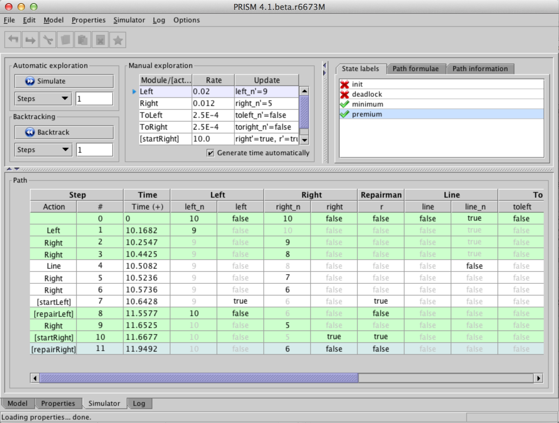
It is also possible to:
Notice that the table containing the path displays not just the value of each variable in each state but also the time spent in that state and any rewards accumulated there. You can configure exactly which columns appear by right-clicking on the path and selecting "Configure view". For rewards (and for CTMC models, for the time-values), you can can opt to display the reward/time for each individual state and/or the cumulative total up until each point in the path.
At the top-right of the interface, any labels contained in the currently loaded model/properties file are displayed, along with their value in the currently selected state of the path. In addition, the built-in labels "init" and "deadlock" are also included. Selecting a label from the list highlights all states in the current path which satisfy it.
The other tabs in this panel allow the value of path operators (taken from properties in the current file) to be viewed for the current path, as well as various other statistics.
Another very useful feature for some models is to use the "Plot new path" option from the simulator, which generates a plot of some/all of the variable/reward values for a particular randomly generated path through the model.
It is also possible to generate random paths through a model using the command-line version of PRISM. This is achieved using the -simpath switch, which requires two arguments, the first describing the path to be generated and the second specifying the file to which the path should be output (as usual, specifying stdout sends output to the terminal). The following examples illustrate the various ways of generating paths in this way:
These generate a path of 10 steps, a path of at least 7.5 time units and a path ending in deadlock, respectively.
Here's an example of the output:
This shows the sequence of states in the path, i.e. the values of the variables in each state. In the example above, there are 4 variables: s, a, s1 and s2.
The first three columns show the type of transition taken to reach that state, its index within the path (starting from 0) and the time at which it was entered. The latter is only shown for continuous time models. The type of the transition is written as [act] if action label act was taken, and as module1 if the module named module1 takes an unlabelled transition).
Further options can also be appended to the first parameter. For example, option probs=true also displays the probability/rate associated with each transition. For example:
In this example, the rate is 200.0 for all transitions.
To show the state/transition rewards for each step, use option rewards=true.
If you are only interested in values of certain variables of your model, use the vars=(...) option. For example:
Note the use of single quotes around the path description argument to prevent the shell from misinterpreting special characters such as "(".
Notice also that the above only displays states in which the values of some variable of interest changes. This is achieved with the option changes=true, which is automatically enabled when you use vars=(...). If you want to see all steps of the path, add the option changes=false.
An alternative way of viewing paths is to only display paths at certain fixed points in time. This is achieved with the snapshot=x option, where x is the time step. For example:
You can also use the sep=... option to specify the column separator. Possible values are space (the default), tab and comma. For example:
When generating paths to a deadlock state, additional repeat=... option is available which will construct multiple paths until a deadlock is found. For example:
By default, the simulator detects deterministic loops in paths (e.g. if a path reaches a state from which there is a just a single self-loop leaving that state) and stops generating the path any further. You can disable this behaviour with the loopcheck=false option. For example:
One final note: the -simpath switch only generates paths up to the maximum path length setting of the simulator (the default is 10,000). If you want to generate longer paths, either change the
default setting or override it temporarily from the command-line using the -simpathlen switch.
You might also use the latter to decrease the setting,
e.g. to look for a path leading to a deadlock state,
but only within 100 steps:
If required, once the model has been constructed, it can be exported, either for manual examination or for use in another tool. The following can all be exported:
From the command-line version of PRISM, the most convenient and flexible approach is to use the -exportmodel switch.
This will, by default, use the extension of the filename(s) to determine the format.
From the GUI, use the "Model | Export" menu to export the data to a file or, for small models, use the "Model | View" menu to print the details directly to the log. For the case of labels, if you want to export labels from the properties file too, use the "Properties | Export labels" option, rather than the "Model | Export" one.
The main formats for model export are:
This format exports different parts of the model in different file, with the expected filename extensions being:
.tra - transition matrix
.srew, .trew, .rew - rewards: states, transitions or both
.lab - labels
.sta - states
.obs - observations
To export just the transition matrix in this format, use:
To export multiple parts, use, e.g.:
If you omit the file basename of the export files and the basename of the model will be used, so this is equivalent to the above:
You can use the shorthand .all to export everything, and .rew to export both state and transition rewards. For example:
You can always use stdout instead of a filename. For example:
is a quick way to print all details (of a small model) to the terminal.
The labels (.lab) export includes the built-in labels "init" and "deadlock",
providing a way to export information about initial states and (fixed) deadlock states.
When there are multiple reward structures, a separate file is created for each one and a (1-indexed) suffix is added to distinguish them. By default, a header in each file (see the "Explicit Model Files" appendix) also shows the name of the reward structure. This can be omitted - see the options below - or via the option "Include headers in model exports" in the GUI.
UMB is a binary format that can incorporate all parts of the model listed above.
By default, everything is included. You can omit some parts with the -exportmodel
options rewards, labels, states and obs, e.g.:
For a small model, you can also see a textual version of the UMB format
using file extension .umbt (or option text):
You can also configure the compression used: zip=false turns it off,
zip=gzip uses gzip and zip=xz uses xz (smaller but slower to read/write).
If the file extension is not recognised, PRISM defaults to plain text (explicit) format. You can always override this using the @format@ option, e.g.:
You can perform multiple model exports using several instances of -exportmodel, e.g.:
Other file formats are also available:
.m) or format=matlab
.drn) or format=drn
Other -exportmodel options are:
actions (=true/false) - whether to actions on choices/transitions
precision (=<n>) - use <n> significant figures for floating point values (in text)
headers (=true/false) - whether to include headers when exporting rewards
rows - export matrices with one row/distribution on each line (plain text)
proplabels - also export labels from a properties file into a .lab file
For plain text export, although -exportmodel is now usually the best switch to use,
other older switches still exist. For example, you can export individual files using
-exporttrans <file>,
-exportstates <file>,
-exportstaterewards <file>,
-exporttransrewards <file>,
-exportrewards <file> <file>,
-exportlabels <file>, and
-exportproplabels <file>.
And you can use switches
-exportmodelprecision <x>,
-exportmatlab and
-exportrows
to specify format options affecting all of them.
It is also possible to export the set of (bottom) strongly connected components (SCCs or BSCCs) for a model. This can only be done from the command-line currently. Use, for example:
For an MDP, you can also export the set of maximal end components (MECs):
Typically, once a model has been constructed, it is analysed through model checking.
Properties are specified as described in the "Property Specification" section,
and are usually kept in files with extensions .props, .pctl or .csl.
There are properties files accompanying most of the sample PRISM models in the prism-examples directory.
To load a file containing properties into the GUI, select menu option "Properties | Open properties list". The file can only be loaded if there are no errors, otherwise an error is displayed. Note that it may be necessary to have loaded the corresponding model first, since the properties will probably make reference to variables (and perhaps constants) declared in the model file. Once loaded, the properties contained in the file are displayed in a list in the "Properties" tab of the GUI. Constants and labels are displayed in separate lists below. You can modify or create new properties, constants and labels from the GUI, by right-clicking on the appropriate list and selecting from the pop-up menu which appears. Properties with errors are shaded red and marked with a warning sign. Positioning the mouse pointer over the property displays the corresponding error message.
The pop-up menu for the properties list also contains a "Verify" option,
which allows you instruct PRISM to model check the currently selected properties
(hold down Ctrl/Cmd to select more than one property simultaneously).
All properties can be model checked at once by selecting "Verify all".
PRISM verifies each property individually.
Upon completion, the icon next to the property changes according to the result of model checking. For Boolean-valued properties, a result of true or false is indicated by a green tick or red cross, respectively. For properties which have a numerical result (e.g. P=? [ ...]), position the mouse pointer over the property to view the result.
In addition, this and further information about model checking is displayed in the log in the "Log" tab.
From the command-line, model checking is achieved by passing both a model file and a properties file as arguments, e.g.:
The results of model checking are sent to the display and are as described above for the GUI version.
By default, all properties in the file are checked.
To model check only a single property, use the -prop switch.
For example, to check only the fourth property in the file:
or to check only the property with name "safe" in the file:
You can also provide a comma-separated list of multiple properties to check, using neither numerical indices or property names:
Alternatively, the contents of a properties file can be specified directly from the command-line, using the -pf switch:
The switches -pctl and -csl are aliases for -pf.
Note the use of single quotes ('...') to avoid characters such as
( and > being interpreted by the command-line shell.
Single quotes are preferable to double quotes since PRISM properties often include double quotes, e.g. for references to labels or properties.
The discrete-event simulator built into PRISM (see the section "Debugging Models With The Simulator") can also be used to generate approximate results for PRISM properties, a technique often called statistical model checking. Essentially, this is achieved by sampling: generating a large number of random paths through the model, evaluating the result of the given properties on each run, and using this information to generate an approximately correct result. This approach is particularly useful on very large models when normal model checking is infeasible. This is because discrete-event simulation is performed using the PRISM language model description, without explicitly constructing the corresponding probabilistic model.
Currently, statistical model checking can only be applied to P or R operators
and does not support LTL-style path properties or filters.
There are also a few restrictions on the modelling language features that can be used; see below for details.
To use this functionality, load a model and some properties into PRISM, as described in the previous sections. To generate an approximate value for one or more properties, select them in the list, right-click and select "Simulate" (as opposed to "Verify"). As usual, it is first necessary to provide values for any undefined constants. Subsequently, a dialog appears. Here, the state from which approximate values are to be computed (i.e. from which the paths will be generated) can be selected. By default, this is the initial state of the model. The other settings in the dialog concern the methods used for simulation.
PRISM supports four different methods for performing statistical model checking:
The first three of these are intended primarily for "quantitative" properties (e.g. of the form P=?[...]), but can also be used for "bounded" properties (e.g. of the form P<p[...]). The SPRT method is only applicable to "bounded" properties.
Each method has several parameters that control its execution, i.e. the number of samples that are generated and the accuracy of the computed approximation. In most cases, these parameters are inter-related so one of them must be left unspecified and its value computed automatically based on the others. In some cases, this is done before simulation; in others, it must be done afterwards.
Below, we describe each method in more detail.
For simplicity, we describe the case of checking a P operator.
Details for the case of an R operator can be found in [Nim10].
The CI method gives a confidence interval for the approximate value generated for a P=? property, based on a given confidence level and the number of samples generated.
The parameters of the method are:
Let X denote the true result of the query P=?[...] and Y the approximation generated.
The confidence interval is [Y-w,Y+w], i.e. w gives the half-width of the interval.
The confidence level, which is usually stated as a percentage, is 100(1-alpha)%.
This means that the actual value X should fall into the confidence interval [Y-w,Y+w] 100(1-alpha)% of the time.
To determine, for example, the width w for given alpha and N, we use w = q * sqrt(v / N) where q is a quantile, for probability 1-alpha/2, from the Student's t-distribution with N-1 degrees of freedom and v is (an estimation of) the variance for X. Similarly, we can determine the required number of iterations, from w and alpha, as N = (v * q2)/w2, where q and v are as before.
For a bounded property P~p[...], the (Boolean) result is determined according to the generated approximation for the probability. This is not the case, however, if the threshold p falls within the confidence interval [Y-w,Y+w], in which case no value is returned.
The ACI method works in exactly same fashion as the CI method, except that it uses the Normal distribution to approximate the Student's t-distribution when determining the confidence interval. This is appropriate when the number of samples is large (because we can get a reliable estimation of the variance from the samples) but may be less accurate for small numbers of samples.
The APMC method, based on [HLMP04], offers a probabilistic guarantee on the accuracy of the approximate value generated for a P=? property, based on the Chernoff-Hoeffding bound.
The parameters of the method are:
Letting X denote the true result of the query P=?[...] and Y the approximation generated, we have:
where the parameters are related as follows: N = ln(2/delta) / 2epsilon2. This imposes certain restrictions on the parameters, namely that N(epsilon2) ≥ ln(2/delta)/2.
In similar fashion to the CI/ACI methods, the APMC method can be also be used for bounded properties such as P~p[...], as long as the threshold p falls outside the interval [Y-epsilon,Y+epsilon].
The SPRT method is specifically for bounded properties, such as P~p[...] and is based on acceptance sampling techniques [YS02]. It uses Wald's sequential probability ratio test (SPRT), which generates a succession of samples, deciding on-the-fly when an answer can be given with a sufficiently high confidence.
The parameters of the method are:
Consider a property of the form P≥p[...]. The parameter delta is used as the half-width of an indifference region [p-delta,p+delta]. PRISM will attempt to determine whether either the hypothesis P≥(p+delta)[...] or P≤(p-delta)[...] is true, based on which it will return either true or false, respectively. The parameters alpha and beta represent the probability of the occurrence of a type I error (wrongly accepting the first hypothesis) and a type II error (wrongly accepting the second hypothesis), respectively. For simplicity, PRISM assigns the same value to both alpha and beta.
Another setting that can be configured from the "Simulation Parameters" dialog is the maximum length of paths generated by PRISM during statistical model checking. In order to perform statistical model checking, PRISM needs to evaluate the property being checked along every generated path. For example, when checking P=? [ F<=10 "end" ], PRISM must check whether F<=10 "end" is true for each path. On this example (assuming a discrete-time model), this can always be done within the first 10 steps. For a property such as P=? [ F "end" ], however, there may be paths along which no finite fragment can show F "end" to be true or false. So, PRISM imposes a maximum path length to avoid the need to generate excessively long (or infinite) paths.
The default maximum length is 10,000 steps.
If, for a given property, statistical model checking results in one or more paths on which the property cannot be evaluated, an error is reported.
Statistical model checking can also be enabled from the command-line version of PRISM, by including the -sim switch. The default methods used are CI (Confidence Interval) for "quantitative" properties and SPRT (Sequential Probability Ratio Test) for "bounded" properties. To select a particular method, use switch -simmethod <method> where <method> is one of ci, aci, apmc and sprt. For example:
PRISM has default values for the various simulation method parameters, but these can also be specified using the switches -simsamples, -simconf, -simwidth and -simapprox. The exact meaning of these switches for each simulation method is given in the table below.
| CI | ACI | APMC | SPRT | |
-simsamples | "Num. samples" | "Num. samples" | "Num. samples" | n/a |
-simconf | "Confidence" | "Confidence" | "Confidence" | "Type I/II error" |
-simwidth | "Width" | "Width" | n/a | "Indifference" |
-simapprox | n/a | n/a | "Approximation" | n/a |
The maximum length of simulation paths is set with switch -simpathlen.
Currently, the simulator does not support every part of the PRISM modelling languages. For example, it does not handle models with multiple initial states or with system...endsystem definitions.
It is also worth pointing out that statistical model checking techniques are not well suited to models that exhibit nondeterminism, such as MDPs. This because the techniques rely on generation of random paths, which are not well defined for a MDP. PRISM does allow statistical model checking to be performed on an MDP, but does so by simply resolving nondeterministic choices in a (uniformly) random fashion (and displaying a warning message). Currently PTAs are not supported by the simulator.
If the model is a CTMC or DTMC, it is possible to compute corresponding vectors of
steady-state or transient probabilities directly
(rather than indirectly by analysing a property which requires their computation).
From the GUI, select an option from the "Model | Compute" menu.
For transient probabilities, you will be asked to supply the
time value for which you wish to compute probabilities.
From the command-line, add the -steadystate (or -ss) switch:
for steady-state probabilities or the -transient (or -tr) switch:
for transient probabilities, again specifying a time value in the latter case. The probabilities are computed for all states of the model and displayed, either on the screen (from the command-line) or in the log (from the GUI).
To instead export the vector of computed probabilities to a file, use the "Model | Compute/export" option from the GUI, or the -exportsteadystate (or -exportss) and -exporttransient (or -exporttr) switches from the command-line:
From the command-line, you can request that the probability vectors exported are in Matlab format by adding the -exportmatlab switch.
By default, for both steady-state and transient probability computation,
PRISM assumes that the initial probability distribution of the model is
an equiprobable choice over the set of initial states.
You can override this and provide a specific initial distribution. This is done using the -importinitdist switch. The format for this imported distribution is identical to the ones exported by PRISM, i.e. simply a list of probabilities for all states separated by new lines. For example, this:
is (essentially) equivalent to this:
Finally, you can compute transient probabilities for a range of time values, e.g.:
which computes transient probabilities for the time points 0.1, 0.11, 0.12, .., 0.2. In this case, the computation is done incrementally, with probabilities for each time point being computed from the previous point for efficiency.
PRISM supports experiments, which is a way of automating multiple instances of model checking. This is done by leaving one or more constants undefined, e.g.:
This can be done for constants in the model file, the properties file, or both.
Before any verification can be performed, values must be provided for any such constants. In the GUI, a dialog appears in which the user is required to enter values. From the command line, the -const switch must be used, e.g.:
To run an experiment, provide a range of values for one or more of the constants. Model checking will be performed for all combinations of the constant values provided. For example:
where N=4:6 means that values of 4,5 and 6 are used for N,
and T=60:10:100 means that values of 60, 70, 80, 90 and 100 (i.e. steps of 10) are used for T.
For convenience, constant specifications can be split across separate instances of the -const switch, if desired.
You can also specify double-valued constants as fractions rather than decimals. For example:
From the GUI, the same thing can be achieved by selecting a single property, right clicking on it and selecting "New experiment" (or alternatively using the popup menu in the "Experiments" panel). Values or ranges for each undefined constant can then be supplied in the resulting dialog. Details of the new experiment and its progress are shown in the panel. To stop the experiment before it has completed, click the red "Stop" button and it will halt after finishing the current iteration of model checking. Once the experiment has finished, right clicking on the experiment produces a pop-up menu, from which you can view the results of the experiment or export them to a file.
For experiments based on properties which return numerical results, you can also use the GUI to plot graphs of the results. This can be done either before the experiment starts, by selecting the "Create graph" tick-box in the dialog used to create the experiment (in fact this box is ticked by default), or after the experiment's completion, by choosing "Plot results" from the pop-up menu on the experiment. A dialog appears, where you can choose which constant (if there are more than one) to use for the x-axis of the graph, and for which values of any other constants the results should be plotted. The graph will appear in the panel below the list of experiments. Right clicking on a graph and selecting "Graph options" brings up a dialog from which many properties of the graph can be configured. From the pop-up menu of a graph, you can also choose to print the graph (to a printer or Postscript file) or export it in a variety of formats: as an image (PNG or JPEG), as an encapsulated Postscript file (EPS), in an XML-based format (for reloading back into PRISM), or as code which can be used to generate the graph in Matlab.
Approximate computation of quantitive results obtained with the simulator can also be used on experiments. In the GUI, select the "Use Simulation" option when defining the parameters for the experiment. From the command-line, just add the -sim switch as usual.
You can export all the results from an experiment to a file or to the screen. From the command-line, use the -exportresults switch, for example:
to send to output file res.txt, or:
to send the results straight to the screen. From the GUI, right click on the experiment and select "Export results".
The default behaviour is to export a list of results in text form, using tabs to separate items. The above examples produce:
You can change the format in which the results are exported by appending one or more comma-separated options to the end of the -exportresults switch, for example to export in CSV (comma-separated values) format:
or in DataFrame format:
You can also add the matrix option, to export the results as one or more 2D matrices, rather than a list.
This is particularly useful if you want to create a surface plot from results that vary over two constants.
The matrix option is also available in normal (non-CSV) mode.
You can also export results in the form of comments, used by PRISM's regression testing functionality:
From the GUI, it is also possible to import previously exported results (in DataFrame format).
A related option is the -exportvector <file> switch, useful in general contexts, not for experiments.
This exports the results for all states of the model
(typically, the log just displays the result for the initial state, unless a filter has been used)
to the the file file.
Properties to be model checked on MDPs (and their variants, such as POMDPs or IMDPs) usually quantify over strategies (or policies) of the model, i.e., over the different possible ways that nondeterminism can be resolved in the model. For example, this property:
determines the maximum probability, over all strategies, of reaching a state satisfying the label "goal". When checking such properties, you can also ask PRISM to generate a corresponding (optimal) strategy, which yields this maximum probability when followed. The strategy can then be viewed, exported or simulated.
Note: For consistency across models, PRISM now uses the terminology strategy (rather than alternatives such as policy). In older versions of the tool, these were referred to as adversaries. Currently, the newer (and more extensive) strategy generation functionality is implemented just for the "explicit" model checking engine, which is used automatically if strategy generation is requested. The old adversary generation functionality (see below) still exists for the "sparse" engine, but will be updated in the future.
Generating strategies. Optimal strategies can be generated either from the command-line or the graphical user interface (GUI). For the former, use the -exportstrat switch. Simple examples are:
From the GUI, you can trigger strategy generation by ticking the "Generate strategy" box either on the popup menu that appears when you right-click a property, or from the "Strategies" menu at the top. As long as it is supported, a strategy will be then generated once "Verify" is clicked.
From the same menu(s), you can then
Strategy export types. Strategies can be viewed or exported in several different formats:
(i) Action list. This is a list of the action taken in each state of the model, e.g.:
where states, by default, are shown as a tuple of variable values.
(ii) Induced model. This is a representation of the model that is induced when the strategy is applied. There are two "modes" for this export. The first (and default) is
reduce, which removes the nondeterminism resolved by the strategy (e.g., an MDP becomes a DTMC). This can be useful to re-import the model back into PRISM and analyse the induced model. The second is restrict, which shows the original model but with a restricted set of choices (e.g., an MDP with just one choice in each state). In each case, the transitions of the induced model are presented as a .tra file (as for normal model export), e.g.:
(iii) Dot file. This is, like the previous format, a view of the model induced by the strategy, but in Dot format, which allows it to be visualised.
Configuring strategy export.
As hinted in the command-line examples above, the -exportstrat switch uses the file extension to determine the preferred format: if the strategy is exported to a file with extension .tra or .dot, then it uses an induced model or Dot file, respectively. Otherwise, the default is an action list. You can specify the desired format:
Further options can be added, e.g., to specify whether an induced model is exported in "restrict" or "reduce" mode:
A full list of available options is as follows:
type (actions, induced or dot): the type of strategy export to use (action list, induced model or Dot file)
mode (restrict or reduce): when exporting as an induced model or Dot file, whether to "restrict" or "reduce" the model (see above); the default is "restrict"
reach (true or false): whether to restrict the strategy to states that are reachable when it is applied to the model (this is currently only used for exporting induced models and Dot files, and the default value is false and true, respectively, in these two cases)
states (true or false): whether to show states, rather than state indices, for actions lists or Dot files; this is true by default
obs (true or false): for partially observable models, whether to merge observationally equivalent states; this is true by default
Strategy types. PRISM generates several types of strategies. The simplest are memoryless deterministic strategies, which pick a single action in each state, as in the examples above. For some query types (e.g., step-bounded properties, or LTL-based properties), finite-memory strategies are generated, where an additional memory value is used. For these, induced models or Dot files are most useful since they will also show how the memory values are updated as the strategy is executed. Note that, in these cases, the state indices of the strategy will correspond to the product model constructed during model checking, not the original model. The product model can be exported using the -exportprodtrans and -exportprodstates switches.
Adversary generation. As mentioned above, the "sparse" model checking engine still includes older so-called "adversary generation" functionality. This can be used to export the induced model to a file using the -exportadv switch, e.g.:
where the -exportadv and -exportadvmdp export a DTMC and an MDP, respectively, i.e., corresponding to the "reduce" and "restrict" modes described above.
From the GUI, change the "Adversary export" option (under the "PRISM" settings) from "None" to "DTMC" or "MDP". You can also change the filename for the export adversary which, by default, is adv.tra as in the example above.
For CTMCs, PRISM also accepts model descriptions in the stochastic process algebra PEPA [Hil96]. The tool compiles such descriptions into the PRISM language and then constructs the model as normal. The language accepted by the PEPA to PRISM compiler is actually a subset of PEPA. The restrictions applied to the language are firstly that component identifiers can only be bound to sequential components (formed using prefix and choice and references to other sequential components only). Secondly, each local state of a sequential component must be named. For example, we would rewrite:
as:
Finally, active/active synchronisations are not allowed since the PRISM
definition of these differs from the PEPA definition. Every PEPA
synchronisation must have exactly one active component.
Some examples of PEPA model descriptions which can be imported into PRISM
can be found in the prism-examples/pepa directory.
From the command-line version of PRISM, add the -importpepa switch and the model will be treated as a PEPA description.
From the GUI, select "Model | Open model" and then choose "PEPA models"
on the "Files of type" drop-down menu.
Alternatively, select "Model | New | PEPA model" and either type a description from scratch
or paste in an existing one from elsewhere.
Once the PEPA model has been successfully parsed by PRISM,
you can view the corresponding PRISM code (as generated by the PEPA-to-PRISM compiler)
by selecting menu option "Model | View | Parsed PRISM model".
PRISM includes a (prototype) tool to translate specifications in SBML (Systems Biology Markup Language) to model descriptions in the PRISM language. SBML is an XML-based format for representing models of biochemical reaction networks. The translator currently works with Level 2 Version 1 of the SBML specification, details of which can be found here.
Since PRISM is a tool for analysing discrete-state systems, the translator is designed for SBML files intended for discrete stochastic simulation. A useful set of such files can be found in the CaliBayes Discrete Stochastic Model Test Suite. There are also many more SBML files available in the BioModels Database.
We first give a simple example of an SBML file and its PRISM translation. We then give some more precise details of the translation process.
An SBML file comprises a set of species and a set of reactions which they undergo. Below is the SBML file for the simple reversible reaction: Na + Cl ↔ Na+ + Cl-, where there are initially 100 Na and Cl atoms and no ions, and the base rates for the forwards and backwards reactions are 100 and 10, respectively.
And here is the resulting PRISM code:
From the latter, we can use PRISM to generate a simple plot of the expected amount of Na and Na+ over time (using both model checking and a single random trace from the simulator):
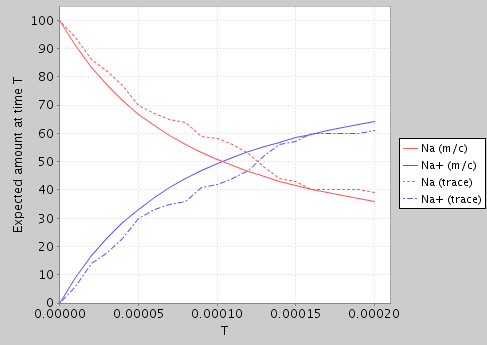
At present, the SBML-to-PRISM translator is included in the PRISM code-base, but not integrated into the application itself.
If you are using a binary (rather than source code) distribution of PRISM, replace classes with lib/prism.jar in the above.
Alternatively (on Linux or Mac OS X), ensure prism is in your path and then save the script below as an executable file called sbml2prism:
Then use:
The following PRISM properties file will also be useful:
This contains a single property which, based on the reward structures in the PRISM model generated by the translator, means "the expected amount of species c at time T". The constant c is an integer index which can range between 1 and N, where N is the number of species in the model. To view the expected amount of each species over time, create an experiment in PRISM which varies c from 1 to N and T over the desired time range.
The basic structure of the translation process is as follows:
boundaryCondition flag is set to true in the SBML file do not have a corresponding module.
reaction_rates stores the expression representing the rate of each reaction (from the corresponding kineticLaw section in the SBML file). Reaction stoichiometry information is respected but must be provided in the scalar stoichiometry field of a speciesReference element, not in a separate StoichiometryMath element.
As described above, this translation process is designed for discrete systems and so the amount of each species in the model is represented by an integer variable. It is therefore assumed that the initial amount for each species specified in the SBML file is also given as an integer. If this is not the case, then the values will need to be scaled accordingly first.
Furthermore, since PRISM is primarily a model checking (rather than simulation) tool, it is important that the amount of each species also has an upper bound (to ensure a finite state space). When model checking, the efficiency (or even feasibility) of the process is likely to be very sensitive to the upper bound(s) chosen. When using the discrete-event simulation functionality of PRISM, this is not the case and the bounds can can be set much higher. By default the translator uses an upper bound of 100 (which is increased if the initial amount exceeds this). A different value can specified through a second command-line argument as follows:
Alternatively, upper bounds can be modified manually after the translation process.
Finally, The following aspects of SBML files are not currently supported and are ignored during the translation process:
It is also possible to construct models in PRISM through direct specification of their transition matrix. Two formats for explicit model import are currently supported:
.tra" files)
Presently, this functionality is only supported in the command-line version of the tool, usually using the -importmodel switch.
In a similar fashion to -exportmodel switch, the type of import is usually determined from the file extension.
For UMB, all model info is contained in a single file. An example of import is:
For the plain text files (.tra etc.), various options are possible.
To just import the core part of the model (the transition function) use:
PRISM tries to determine the model type from the format of the .tra file,
but if this does not work, the model type can be overwritten using the -dtmc, -ctmc and -mdp switches.
For example:
Using the same formats as for model export, other parts of the model can also be imported:
.lab - labels
.srew, .trew - rewards: states, transitions
.sta - states
.obs - observations
Here is an example of also importing labels and states:
If state information is not imported, a single zero-indexed variable x is assumed.
Note also that, since details about the initial state(s) of a model are not preserved in the .tra file,
but are included in the labels file, this should also be used to designate a particular initial state for a model.
Otherwise, state 0 is assumed to be the initial state or,
if state information is imported, the state in which all variables take their minimum value is used.
Use the extension .all to import from any matching files with appropriate extensions:
In this case, you can omit the -importmodel switch and just specify the .all-ended filename, e.g.:
Please note, for PRISM's symbolic model construction/engines, which are often used by default, this explicit method of constructing models in PRISM is typically less efficient than using the PRISM language. This is because the underlying data structures used to represent the model function better when there is high-level structure and regularity to exploit. You may want to switch to the "explicit" engine:
The situation can also be alleviated to a certain extent for the symbolic implementations by importing
the .sta file, since the composition of the states reintroduces some regularity
(although is still typically inefficient to construct).
In a similar style to PRISM's -exportmodel switch, while -importmodel is usually the most convenient, you can also specify each part separately, e.g.:
There are also -importstaterewards and -impottransrewards switches.
You can import multiple reward structures using multiple instances of the these switches.
If present in the rewards files (see the appendix "Explicit Model Files"),
the names of the reward structures are read too.
The operation of PRISM can be configured in a number of ways. From the GUI, select "Options" from the main menu to bring up the "Options" dialog. The settings are grouped under several tabs. Those which affect the basic model checking functionality of the tool are under the heading "PRISM". Separate settings are available for the simulator and various aspects of the GUI (the model editor, the property editor and the log).
User options and settings for the GUI are saved in a file locally and reused. Currently the "Options" dialog in the GUI represents the easiest way to modify the settings, but the settings file is in a simple textual format and can also be edited by hand. To restore the default options for PRISM, click "Load Defaults" and then "Save Options" from the "Options" dialog in the GUI. Alternatively, delete the settings file re-launch the GUI. The location of the settings file depends on the operating system. As of PRISM 4.5, it is stored in:
$HOME/.prism (if the settings file was already created by an older version of PRISM)
$XDG_CONFIG_HOME/prism.settings (on Linux, if that environment variable is set)
$HOME/.config/prism.settings (on Linux, if $XDG_CONFIG_HOME is not set)
$HOME/Library/Preferences/prism.settings (on Mac OS)
.prism in the user's home directory, e.g. C:\Documents and Settings\username (on Windows)
From the command-line version of PRISM, options are controlled by switches. A full list can be displayed by typing:
For some switches, whose format is not straightforward, there is additional help available on the command-line, using -help switch. For example:
The settings file is ignored by the command-line version (unlike earlier versions of PRISM, where it was used). You can, however, request that the settings file is read, using the -settings switch, e.g.:
In the following sections, we give a brief description of the most important configuration options available.
PRISM contains four main engines, which implement the majority of its model checking functionality:
The first three of these engines are either wholly or partly symbolic, meaning that they use data structures such as binary decision diagrams (BDDs) and multi-terminal BDDs (MTBDDs). For these three engines, the process of constructing a probabilistic model (DTMC, MDP or CTMC) is performed in a symbolic fashion, representing the model as an MTBDD. Subsequent numerical computation performed during model checking, however, is carried out differently for the three engines. The "MTBDD" engine is implemented purely using MTBDDs and BDDs; the "sparse" engine uses sparse matrices; and the "hybrid" engine uses a combination of the other two. The "hybrid" engine is described in [KNP04b]. For detailed information about all three engines, see [Par02].
The fourth engine, "explicit", performs all aspects of model construction and model checking using explicit-state data structures. Models are typically stored as sparse matrices or variants of. This engine is implemented purely in Java, unlike the other engines which make use of code/libraries implemented in C/C++. One goal of the "explicit" engine is to provide an easily extensible model checking engine without the complication of symbolic data structures, although it also has other benefits (see below).
The choice of engine ("MTBDD", "sparse", "hybrid" or "engine") should not affect the results of model checking - all engines perform essentially the same calculations. In some cases, though, certain functionality is not available with all engines and PRISM will either automatically switch to an appropriate engine, or prompt you to do so. Performance (time and space), however, may vary significantly and if you are using too much time/memory with one engine, it may be worth experimenting. Below, we briefly summarise the key characteristics of each engine.
When using the PRISM GUI, the engine to be used for model checking can be selected from the "Engine" option under the "PRISM" tab of the "Options" dialog. From the command-line, engines are activated using the -mtbdd, -sparse, -hybrid and -explicit (or -m, -s, -h and -ex, respectively) switches, e.g.:
Note also that precise details regarding the memory usage of the current engine are displayed during model checking (from the GUI, check the "Log" tab). This can provide valuable feedback when experimenting with different engines.
PRISM also has some basic support for automatically selecting the engine (and other settings) heuristically,
based on the size and type of the model, and the property being checked.
Use, for example, -heuristic speed from the command-line to choose options
which target computation speed rather than saving memory.
This is also available from the "Heuristic" option under the "PRISM" tab of the "Options" dialog in the GUI.
Although it is not treated as a separate "engine", like those above,
PRISM also provides approximate/statistical model checking,
which is based on the use of discrete-event simulation.
From the GUI, this is enabled by choosing "Simulate" menu items or tick boxes;
from the command-line, add the -sim switch.
See the "Statistical Model Checking"
section for more details.
Most of PRISM's model checking functionality uses numerical solution based on floating point arithmetic and, often, this uses iterative numerical methods, which are run until some user-specified precision is reached. PRISM currently has some support for "exact" model checking, i.e., using arbitrary precision arithmetic to provide exact numerical values. Currently, this is implemented as a special case of parametric model checking, which limits is application to relatively small models. It can be used for analysing DTMCs/CTMCs (unbounded until, steady-state probabilities, reachability reward and steady-state reward) or MDPs (unbounded until and reachability rewards). You can enable this functionality using the "Do exact model checking" option in the GUI or using switch -exact from the command line.
The techniques used to model check PTAs are different to the ones used for DTMCs, MDPs and CTMCs. For PTAs, PRISM currently has three distinct engines that can be used:
The default engine for PTAs is "stochastic games". The engine to be used can be specified using the "PTA model checking method" setting in the "PRISM" options panel in the GUI. From the command-line, switch -ptamethod <name> should be used where <name> is either games, digital or backwards.
The choice of engine for PTA model checking affects restrictions that imposed on both the modelling language and the types of properties that can be checked.
Separately from the choice of engines, PRISM often offers several different solution methods that can be used for the computation of probabilities and expected costs/rewards during model checking. Many, but not all, of these are iterative numerical methods. The choice of method (and their settings) depends on the type of analysis that is being done (i.e., what type of model and property).
For many properties of Markov chains (e.g. "reachability"/"until" properties for DTMCs and CTMCs, steady-state properties for CTMCs and "reachability reward" properties for DTMCs), PRISM solves a set of linear equation systems, for which several numerical methods are available. Below is a list of the alternatives and the switches used to select them from the command-line. The corresponding GUI option is "Linear equations method".
-power (or -pow, -pwr)
-jacobi (or -jac)
-gaussseidel (or -gs)
-bgaussseidel (or -bgs)
-jor
-sor
-bsor
When using the MTBDD engine, Gauss-Seidel/SOR based methods are not available.
When using the hybrid engine, pseudo variants of Gauss-Seidel/SOR based method can also be used [Par02]
(type prism -help at the command-line for details of the corresponding switches).
For methods which use over-relaxation (JOR/SOR), the over-relaxation parameter (between 0.0 and 2.0)
can also be specified with option "Over-relaxation parameter" (switch -omega <val>).
For options relating to convergence (of this and other iterative methods), see the Convergence section below.
When analysing MDPs, there are multiple solution methods on offer. For most of these, you can select them under the "MDP solution method" setting from the GUI, or use the command-line switches listed below. Currently, all except value iteration are only supported by the explicit engine. For more details of the methods, see e.g. [FKNP11] (about probabilistic verification of MDPs) or classic MDP texts such as [Put94]).
-valiter) [this is the default]
-gs)
-politer)
-modpoliter)
Where the methods above use iterative numerical solution, you can also use the settings under described in the Convergence section below.
Interval iteration [HM14],[BKLPW17] is an alternative solution method for either MDPs or DTMCs
which performs two separate instances of numerical iterative solution,
one from below and one from above. This is designed to provide clearer information
about the accuracy of the computed values and avoid possible problems with premature convergence.
This can be enabled using the switch -intervaliter (or -ii)
or via the "Use interval iteration" GUI option.
A variety of options can be configured, either using
-intervaliter:option1,option2,... or by
setting the string "option1,option2,..." under "Interval iteration options" in the GUI.
Type prism -help intervaliter from the command-line for a list of the options
and see [BKLPW17] for the details.
Topological value iteration is a variant of value iteration which improves efficiency
by analysing the graph structure of the model and using this to update the values for
states in an alternative order which increases the speed of convergence.
Use switch -topological or GUI option "Use topological value iteration" to enable this.
In addition to standard value iteration for MDPs, the topological variant can be used to optimise
both interval iteration (see above) and the numerical solution of DTMCs.
When computing transient probabilities of a CTMC
(either directly or when verifying time-bounded operators of CSL), there are two options:
uniformisation and fast adaptive uniformisation (FAU). These can be selected using the GUI option "Transient probability computation method", or using the command-line switch -transientmethod <name>, where <name> is either unif or fau.
Uniformisation is a standard iterative numerical method for computing transient probabilities on a CTMC, which works by reducing the problem to an analysis of a "uniformised" DTMC.
As an optimisation, when it is detected that the transient probabilities have converged, no further iterations are performed. If necessary (e.g. in case of round-off problems), this optimisation can be disabled with the "Use steady-state detection" option (command-line switch -nossdetect).
Fast adaptive uniformisation (FAU) [MWDH10] is a method to efficiently approximate transient properties of large CTMCs. The basic idea is that only the parts of the model that are relevant for the current time period are kept in memory. In more detail, starting with the initial states, in each step FAU explores further states in a DTMC which is a discrete-time version of the original CTMC. By combining the probabilities there with those of a certain continuous-time stochastic process (a birth process), transient properties in the original CTMC can be computed. If it turns out that the probability of being in some state in the DTMC is below a given threshold, this state is removed from the model explored so far. After a given number of steps, which corresponds to the number of steps which are likely to happen within the time bound, the exploration can be stopped. In the implementation in PRISM [DHK13], FAU can be used to compute transient probability distributions and to model check the following types of non-nested CSL formulas: time-bounded until, instantaneous reward, cumulative reward.
The following options can be used to configure FAU:
-fauepsilon <x>): FAU analyses the DTMC for a number of iterations such that the probability of more steps being relevant is below this value. The default is 1e-6.
-faudelta <x>): States that have a lower probability than this value are discarded. The default is 1e-12.
-fauarraythreshold <x>): After this number of steps without any new states being explored or discarded, FAU will switch to a faster, fixed-size data structure until further states have to be explored or discarded. The default is 100.
-fauintervals <x>): In some cases, it is advantageous to divide the time interval the analysis is done for into several smaller intervals. This option dictates the number of (equal length) intervals used for this split. The default is 1, meaning that only one time interval is used.
-fauinitival <x>): It is also possible to specify an additional initial time interval which is handled separately from the rest of the time. This is often advantageous, because in this interval certain parameters of the model can be explored, which can subsequently be used to speed up the computation of the remaining time interval. The default for this option is 1.0.
Common to all of these methods is the way that PRISM checks convergence, i.e. decides when to terminate the iterative methods because the answers have converged sufficiently. This is done by checking when the maximum difference between elements in the solution vectors from successive iterations drops below a given threshold (or, in the case of interval iteration, if the difference of the elements in the iterations from above and below are below the threshold).
The default value for this threshold is 10-6 but it can be altered with the "Termination epsilon" option (switch -epsilon <val>). The way that the maximum difference is computed can also be varied:
either "relative" or "absolute" (the default is "relative"). This can be changed using the "Termination criteria" option (command-line switches -relative and -absolute, or -rel and -abs for short).
Also, the maximum number of iterations performed is given an upper limit
in order to trap the cases when computation will not converge.
The default limit is 10,000 but can be changed with the "Termination max. iterations" option (switch -maxiters <val>). Computations that reach this upper limit will trigger an error during model checking to alert the user to this fact.
When PRISM performs verification of LTL formulas, it does so by converting the formula into an automaton (such as a deterministic Rabin automaton) and then analysing a larger product model, constructed from the model being verified and the omega automaton. For this reason, the size of the automaton has an important effect on the efficiency of verification.
By default PRISM uses a port of the ltl2dstar library to construct these automata. But it also allows the use of external LTL-to-automata converters producing deterministic automata through support for the Hanoi Omega Automaton (HOA) format. From the command line, an example of this is:
The -ltl2datool switch specifies the location of the program to be executed to perform the LTL-to-automaton conversion. This will be called by PRISM as "exec in-file out-file", where exec is the executable, in-file is the name of a file containing the LTL formula to be converted and out-file is the name of a file where the resulting automaton should be written, in HOA format. Typically, the executable will be a script. Here is a simple example (called as hoa-ltl2dstar-for-prism in the above example), which calls an external copy of ltl2dstar in the required fashion (assuming that the ltl2dstar and ltl2ba executables are located in the current directory or on the PATH).
PRISM is known to work with these HOA-enabled tools:
and contains ready-made scripts for calling them in the etc/scripts/hoa directory of the distribution:
hoa-ltl2dstar-for-prism ltl2tgba, ltl2ba or LTL3BA as the LTL-to-NBA tool as the LTL-to-NBA tool)
hoa-ltl2tgba-for-prism ltl2tgba)
hoa-ltl3dra-for-prism hoa-rabinizer-for-prism ltl2dra)
See the files themselves for details of any configuration required, possible options and for a reminder of the PRISM command-line arguments required.
There is also a hoa-rabinizer-for-prism.bat script for connecting to Rabinizer on Windows.
The -ltl2dasyntax switch is used to specify the textual format for passing the LTL formula to the external converter (i.e., in the file out-file). The options are:
lbt - LBT format
spin - SPIN format
spot - Spot format
rabinizer - Rabinizer format
Typical usage is:
From the GUI, configuring the external LTL converter is done with the two options "Use external LTL->DA tool" and "LTL syntax for external LTL->DA tool".
Another related option is "All path formulas via automata" (command-line switch -pathviaautomata), which forces construction of an automata
when computing the probability of a path formula, even if it is not needed. This is primarily intended for debugging/testing, not regular use.
As mentioned above, PRISM's external LTL-to-automaton interfacing works using the
HOA format
(and, in particular, using the jhoafparser HOA parser.
Currently, PRISM can handle automata in HOA format that are
deterministic and complete, with state-based acceptance.
Automata with transition-based acceptance are converted to state-based acceptance by PRISM.
For DTMC and CTMC model checking, generic acceptance conditions are supported, i.e.,
anything that can be specified as an Acceptance: header in HOA format.
For MDP model checking, currently Rabin and generalized Rabin acceptance
specified via the acc-name: header are supported. See the HOA format specification for details.
To increase the amount of information displayed by PRISM (in particular, to display lists of states and probability vectors), you can use the "Verbose output" option (activated with command-line switch -verbose or -v). To display additional statistics about MTBDDs after model construction, use the "Extra MTBDD information" option (switch -extraddinfo) and, to view MTBDD sizes during the process of reachability, use option "Extra reachability information" (switch -extrareachinfo).
Sometimes, model checking of properties for MDPs requires fairness constraints to be taken into account.
See e.g. [BK98],[Bai98] for more information.
To enable the use of fairness constraints (for P operator properties), use the -fair switch.
By default, when constructing a model, PRISM checks that all probabilities and rates are within acceptable ranges (i.e. are between 0 and 1, or are non-negative, respectively). For DTMCs and MDPs, it also checks that the probabilities sum up to one for each command. These checks are often very useful for highlighting user modelling errors and it is strongly recommended that you keep them enabled, however if you need to disable them you can do so via option "do prob checks?" in the GUI or command-line switch -noprobchecks.
You can also change the level of precision used to check that probabilities sum to 1 using the option "Probability sum threshold" (or command-line switch -sumroundoff.
CUDD, the underlying BDD and MTBDD library used in PRISM has an upper memory limit. By default, this limit is 1 GB. If you are working on a machine with significantly more memory this and PRISM runs out of memory when model checking, it may help to change this. To set the limit, from the command-line, use the -cuddmaxmem switch. For example:
Above, g denotes GB. You can also use m for MB.
You can also the CUDD maximum memory setting from the options panel in the GUI, but you will need to close and restart the GUI (saving the settings as you do) for this to take effect.
The Java virtual machine (JVM) used to execute PRISM also has upper memory limits. Sometimes this limit will be exceeded and you will see an error of the form java.lang.OutOfMemory. To resolve this problem, you can increase this memory limit. On Unix, Linux or Mac OS X platforms, this can done by using the -javamaxmem switch, passed either to the command-line script prism or the GUI launcher xprism. For example:
each set the limit to 4GB. Alternatively, you set the environment variable PRISM_JAVAMAXMEM before running PRISM. For example, under a bash shell:
If you get an error of the form java.lang.StackOverflowError, then you can try increasing the stack size of the JVM.
On Unix, Linux or Mac OS X platforms, this can done by using the -javastack switch or the PRISM_JAVASTACKSIZE environment variable.
Examples are:
or:
If you are running PRISM on Windows you will have to do make adjustments to Java memory manually, by modifying the prism.bat or xprism.bat scripts.
To set the memory to 4GB, for example, add -Xmx4g to the list of arguments in the call to java or javaw at the end of the file.
To change the stack size to 1GB, add -Xss1g.
If you want to pass additional switches to the JVM used to run PRISM, you can use the -javaparams switch.
For example:
By default, PRISM's probabilistic model checking algorithms use an initial precomputation step which uses graph-based techniques to efficient detect trivial cases where probabilities are 0 or 1. This can often result in improved performance and also reduce round-off errors. Occasionally, though, you may want to disable this step for efficiency (e.g. if you know that there are no/few such states and the precomputation process is slow). This can be done with the -nopre switch. You can also disable the individual algorithms for probability 0/1 using switches -noprob0 and -noprob1.
The command-line version of PRISM has a time-out option, specified using the switch -timeout <n>.
This causes the program to exit after <n> seconds if it has not already terminated by that point.
This is particularly useful for benchmarking scenarios where you wish to ignore runs of PRISM that exceed a certain length of time.
When PRISM crashes, the most likely cause is that it has run out of memory. Similarly, if PRISM (or the machine you are running it on) becomes very slow or seems to have stopped responding, this is probably because it is using too much of your machine's memory. Probabilistic model checking, much like other formal verification techniques, can be a very resource-intensive process. It is very easy to create a seemingly simple PRISM model that requires a large amount of time and/or memory to construct and analyse. See some of the other questions in this section for tips on how to avoid this.
The other possibility is that you have found a bug.
If PRISM crashes or freezes whilst not using all/most of the available memory (you can check this with the top command in a Unix/Linux terminal or the Task Manager (via Ctrl-Alt-Delete) on Windows) then please file a bug report.
It depends. First, you need to establish at what point in PRISM's operation, you ran out of memory. If you are running the command-line version of PRISM then the output from the tool so far should give an indication of this. If using the GUI, check the log tab for this information. If PRISM crashed because of its memory usage, the error message can be helpful. If using the GUI, you may need to start the GUI from the command-line to see any error messages.
The two main steps that PRISM typically has to perform are:
Memory usage issues for each of these steps are discussed in separate sections below. In some cases the process performed prior to step 1 (model parsing - reading in a model description in the PRISM language and checking it for correctness) can also be resource intensive. This is also discussed below.
If you are using the simulator to generate approximate model checking results then step 1 (model construction) is not performed and step 2 is carried out very differently. Memory consumption is not usually a problem in this case.
If PRISM has already output this:
but there is no line of the form:
and then you get an error like this:
or like this:
then PRISM ran out of memory whilst trying to construct the model. Model construction in PRISM is performed using BDDs (binary decision diagrams) and MTBDDs (multi-terminal) BDDs which are implemented in the CUDD library. The first thing to try in this case is to increase the amount of memory available to CUDD. See the entry "CUDD memory" in the section "Configuring PRISM - Other Options" for details of this.
If increasing this memory limit does not resolve the problem, then you will need to consider ways to reduce the size of your model. You can find some tips on this in the PRISM Modelling section. Bear in mind also that if you are having to increase the CUDD memory limit too high (e.g. close to the physical memory available on your computer) just for model construction, then it is unlikely that you will have enough memory for subsequent model checking operations.
Finally, it is also worth considering the ordering of the modules and variables in your model since this can have a (in some cases dramatic) effect on the size of MTBDD representation of the model. This topic is covered in the "PRISM Modelling" section of this FAQ.
If model construction was successfully completed (see previous question) but model checking was not, there are several things you can try. First of all, if the error message you see looks like the one in the previous question or you see a message such as
then it may be worth increasing the memory limit for CUDD (as described above). However, if you see an error more like this:
then increasing the memory CUDD probably will not help - PRISM is just trying to allocate more memory than is physically available on your system.
Here are some general tips:
This is a less common problem and will only occur if the actual PRISM language description of your model is very large. This may be the case, for example, if you are automatically generating PRISM models in some way. Errors due to lack of memory during parsing usually look like:
or:
You can resolve this problem by increasing the memory allocated to Java. See the entry "Java memory" in the section "Configuring PRISM - Other Options" for details of this.
There is no definitive answer to this. Because of PRISM's symbolic implementation, using data structures based on binary decision diagrams (BDDs), its performance can be unpredictable in this respect. There are also several factors that affect performance, including the type of model and property being checked and the engine being used (PRISM has several different engines, which have varying performance).
Having said that, using the default engine in PRISM (the �hybrid� engine), you can normally expect to be able to handle models with up to 10^7-10^8 states on a typical PC. Using the MTBDD engine, you may be able to analyse much larger models (on some of the PRISM case studies, for example, PRISM can do numerical analysis of models with as many as 10^10 or 10^11 states). The manual has more information about PRISM's engines.
The size of a probabilistic model (i.e. the number of states/transitions) is critical to the efficiency of performing probabilistic model checking on it, since both the time and memory required to do so are often proportional to the model size. Unfortunately, it is very easy to create models that are extremely large. Below are a few general tips for reducing model size.
Because PRISM is a symbolic model checker, the amount of memory required to store the probabilistic model can vary (sometime unpredictably) according to several factors. One example is the order in which the variables of your model appear in the model file. In general, there is no definitive answer to what the best ordering is but the following heuristics are a good guide.
Variables x and y are "related" if, for example, the value of one is has an effect on how the other changes (e.g. (y'=x+1)) or if both appear together in an expression (e.g. a guard).
These heuristics also apply to the ordering of modules within the model file.
For technical details about variable ordering issues, see e.g. section 8 of [HKN+03] or section 4.1.2 of [Par02].
All delays in a CTMC need to be modelled as exponential distributions. This is what makes them efficient to analyse. If you included a transition whose delay was deterministic, i.e. which always occurred after exactly the same delay, the model would no longer be a CTMC.
One solution to this, if your model require such a delay, is to approximate a deterministic delay with an Erlang distribution (a special case of a phase-type distribution). See for example this PRISM model:
In the model, the occurrence of the the go-labelled action occurs with an Erlang distribution with mean mean and shape k. The special case of k=1 is just an exponential distribution. The graph below shows the probability distribution of the delay, i.e. of P=? [ F<=T x=1 ] for different values of k.
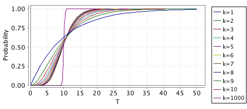
There is an obvious trade-off here between the accuracy (how close it is to modelling a deterministic time delay) and the resulting blow-up in the size of the model that you add this to. For k=1000, you can see that the shape is quite "deterministic" but this would increase your model size by a factor of ~1000.
----
This appendix details the plain text file formats used by PRISM for exporting and importing models that have already been constructed, i.e., they comprise an explicit list of states, transitions, etc. making up the model, rather than a high-level model description in the PRISM modelling language. Below, we describe:
These contain an explicit list of the transitions making up a probabilistic model, i.e. they are essentially a sparse matrix representation of the transition probability/rate matrix. The first line of the file contains information about the size of the model, the remaining lines contain information about transitions, one per line.
DTMCs and CTMCs
For Markov chains the first line take the form "n m", giving the number of states (n) and the number of transitions (m). The remaining lines are of the form "i j x" or "i j x a", where i and j are the indices of the source state (row) and destination state (column) of the transition, and x is the probability (for a DTMC) or rate (for a CTMC) of the transition. State indices are zero-indexed (i.e. between 0 and n-1). Probability/rate values are written as (positive) floating point numbers (examples: 0.5, .5, 5.6e-6, 1). a is optional and gives the action label for the transition. Action labels can be present for some, all or no transitions.
It is assumed that source states (rows) are in ascending order, but there is no assumption about the ordering of destination states (columns) within the transitions for each source state.
For a DTMC, the probabilities for the outgoing transitions of each state should sum to 1.
Here is an example, for the (DTMC) PRISM model lec3.pm (which looks like this):
and here is one for the (CTMC) PRISM model poll2.sm (which looks like this):
MDPs (or PAs)
For MDPs, the format is an extension of the above To clarify terminology: each state of the MDP contains (nondeterministic) choices, each of which is essentially a probability distribution over successor states that we can view as a set of transitions. Optionally, each choice can be labelled with an action.
The first line of the file take the form "n c m", giving the number of states (n), the total number of choices (c) and the total number of transitions (m). The remaining lines are of the form "i k j x" or "i k j x a", where i and j are the indices of the source state (row) and destination state (column) of the transition, k is the index of the choice that it belongs to, and x is the probability of the transition. a is optional and gives the action label for the choice of the transition. Action labels can be present for some, all or no states but, in slightly redundant fashion, the action labels, if present, must be the same for all transitions belonging to the same choice.
State indices and choice indices are all zero-indexed. Probability values (as above) are written as (positive) floating point numbers and should sum to 1 for each choice. It is assumed that source states (rows) and choices within states are in ascending order, but there is no assumption about the ordering of destination states (columns) within the transitions for each choice.
Here is an example, for the (MDP) PRISM model lec12mdp.nm (which looks like this):
and here is an action-labelled version of the same model, lec12mdpa.nm (which looks like this):
POMDPs
The format of a .tra file for a POMDP is similar to an MDP,
but also contains information about observations.
The first line of the file take the form "n c m o", where n, c and m are, as for MDPs, the numbers of states, choices and transitions,
and o is the number of observations.
The lines that list transitions contain an additional integer after the transition probability
(and before the action, if present), giving the (deterministic) observation that is made
when entering the target state of that transition.
Currently, it is assumed that these are consistent for all states.
In order to also specify the observation for the initial state,
a dummy transition line of the form - - s - o is used,
giving both the initial state s and its observation o.
An example file is:
There is alternative format for transition matrices (see the rows option for -exportmodel) where transitions for each state/choice are collated on a single line.
Here is the result for the lec3.pm example from above (a DTMC):
for the lec12mdp.nm example (an MDP):
and for the lec12mdpa.nm example (an MDP with actions):
These contain an explicit list of which labels are satisfied in each state.
The first line lists the labels, assigning each one an index.
The remaining lines list indices of all states satisfying one or more labels,
followed by a list of the the indices of labels that that are satisfied in it.
This includes the built-in labels "init" (initial states) and deadlock (deadlock states).
An example is shown below, where, for example, both "heads" and "end" are satisfied in state 2.
Reward files contain an (optional) header, giving the name of the reward structure that generated it
and the type of rewards (state or transitions) stored in the file.
For state rewards, the information following this header is an explicit list of the (non-zero) state rewards.
The first line is of the form n m where n is the number of states in the model and m is the number of non-zero state rewards.
The following m lines are of the form i r, denoting that the state reward for state i is r.
For the lec3.pm (6-state) DTMC example from above, we get rewards in 3 states (0, 4 and 5):
Files containing transition rewards, like those for state rewards, start with an (optional) header. The rest of the file is formatted identically to transitions files (see above), except that probabilities/rates are replaced with reward values, and the number of transitions (the last number on the first line) is replaced with the number of non-zero transition rewards.
For the lec3.pm (6-state) DTMC example from above, we get non-zero transition rewards on 4 transitions:
And or the lec12mdpa.nm (4-state) MDP example, we get non-zero transition rewards on 4 transitions:
These contain an explicit list of the reachable states of a model. The first line is of the form (v1,...,vn), listing the names of all the variables in the model in the order that they appear in the PRISM model. Subsequent lines list the values of the n variables in each state of the model. Each line is of the form i:(x1,...,xn), where i is the index of the state (starting from 0) and x1,...,xn are the values of each variable in the state. States are ordered by their index (and, therefore, given PRISM's default behaviour, lexicographically according to the tuple of variable values).
For the example PRISM model poll2.sm, the states file looks like:


 Site hosted at the Department of Computer Science, University of Oxford