

Related publications
This case study is based on the distributed energy management algorithm for smart grids by Hildmann & Saffre [HS11]. We performed model checking of the system using PRISM-games, an extension of PRISM with support for stochastic multi-player games. For property specifications, we used the logic rPATL, introduced in [CFK+12, CFK+13b].
Microgrid is an increasingly popular model for the future energy markets where neighbourhoods use electricity generation from local sources (e.g. wind/solar power) to satisfy local demand. The success of microgrids is highly dependent on the active management of demand by users to avoid peaks. Hildmann & Saffre in [HS11] proposed a distributed algorithm which, if followed by the system users, has been show to reduce the peak demand.
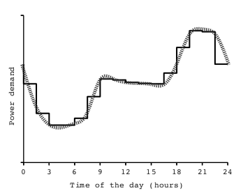
The system in [HS11] consists of N households connected to a single distribution manager. At every time-step, the distribution manager randomly contacts a household for submission of a load for execution. The probability of the household generating a load is determined by a daily demand curve (see below). The duration of a load is chosen uniformly at random between 1 and D time-steps. The cost of executing a load for a single step is the number of tasks currently running. Hence, the total cost increases quadratically with households executing more loads in a single step.
Each household follows a very simple algorithm, the essence of which is that, when it generates a load, if the cost is below an agreed limit clim, it executes it, otherwise it only does so with a pre-agreed probability Pstart. In [HS11], the value for each household in a time-step is measured by V= loads executing⁄cost of execution and it is shown (through simulations) that, provided every household sticks to this algorithm, the peak demand and the total cost of energy are reduced significantly while still providing a good (expected) value V for each household.
We modelled the system as a stochastic multiplayer game (SMG) with N players, one per household. We vary N from 2 to 7 and fix D=4 and clim=1.5. We analyse a period of 3 days, each of 16 time-steps, using a piecewise approximation of the daily demand curve from [HS11]:
The model for three households is shown below.
// Model implementing demand-side energy management algorithm of:
// H. Hildmann and F. Saffre. Influence of Variable Supply and Load Flexibility on Demand-Side Management
// IEEE 8th International Conference on the European Energy Market (EEM). 2011.
//
// In contrast with original (DTMC) model, some agents are allowed to
// make a decision whether to execute their jobs modeled by non-determinism.
//
// Model has to be built using PRISM preprocessor (http://www.prismmodelchecker.org/prismpp/)
// using the following command: prismpp dsm_mdp-dtmc.pp <N> <D> <d> <L> <PS> > dsm_mdp-dtmc.pm, where
//
// <N> - number of households
// <D> - number of days
// <d> - number of deterministic households
// <L> - maximum job duration
// <PS> - 0.Pstart
//
//
// Aistis Simaitis 25/08/11

smg

// number of households
const int N = 3;

// number of days
const int D = 3;

// number of time intervals in the day
const int K = 16;

// expected number of jobs per household per day
const int Exp_J = 9;

// cost limits for households
const double price_limit = 1.5;

// initiation probabilities for jobs (uuniform distribution)
const double P_J1 = 1/4;
const double P_J2 = 1/4;
const double P_J3 = 1/4;
const double P_J4 = 1/4;

// probability of starting a task independently of the cost
const double P_start = 0.8;

// distribution of the expected demand across intervals
const double D_K1 = 0.0614;
const double D_K2 = 0.0392;
const double D_K3 = 0.0304;
const double D_K4 = 0.0304;
const double D_K5 = 0.0355;
const double D_K6 = 0.0518;
const double D_K7 = 0.0651;
const double D_K8 = 0.0643;
const double D_K9 = 0.0625;
const double D_K10 = 0.0618;
const double D_K11 = 0.0614;
const double D_K12 = 0.0695;
const double D_K13 = 0.0887;
const double D_K14 = 0.1013;
const double D_K15 = 0.1005;
const double D_K16 = 0.0762;

// time limit
const int max_time = K*D+1;

// ---------------------------------------------------

// time counter
global time : [1..max_time];

// jobs of households
global job1 : [0..4];
global job2 : [0..4];
global job3 : [0..4];

// scheduling variable
global sched : [0..N];


player p0
 	player0
endplayer

// definition of scheduling module
module player0

	[] sched = 0 -> 1/N : (sched'=1)
		      + 1/N : (sched'=2)
		      + 1/N : (sched'=3)
;

endmodule

// definitions of deterministic households

// definitions of non-deterministic households
player p1
	player1, [start1], [backoff1], [nbackoff1]
endplayer

module player1

	job_arrived1 : [0..4];

	[] sched=1 & active = 0 & job1 > 0 & time < max_time -> (job1'=new_j1) & (job2'=new_j2) & (job3'=new_j3) & (time'=time+1) & (sched'=0);

	// initiate the job with probability P_init
	[] sched=1 & active = 0 & job1 = 0 & time < max_time -> P_init*P_J1 : (job_arrived1'=1)
							    + P_init*P_J2 : (job_arrived1'=2)
							    + P_init*P_J3 : (job_arrived1'=3)
							    + P_init*P_J4 : (job_arrived1'=4)
				       			    + (1-P_init) : (job1'=new_j1) & (job2'=new_j2) & (job3'=new_j3) & (time'=time+1) & (sched'=0);

	// start job if cost below the limit
	[start1] sched=1 & job_arrived1 > 0 & price <= price_limit & time < max_time-> (job1'=job_arrived1)  & (job2'=new_j2) & (job3'=new_j3) & (job_arrived1'=0) & (time'=time+1) & (sched'=0);

	// back-off with probability 1-P_start
	[backoff1] sched=1 & job_arrived1 > 0 & price > price_limit & time < max_time->   P_start : (job1'=job_arrived1)  & (job2'=new_j2) & (job3'=new_j3) & (job_arrived1'=0) & (time'=time+1) & (sched'=0)
						   + (1-P_start) : (job1'=new_j1) & (job2'=new_j2) & (job3'=new_j3) & (job_arrived1'=0) & (time'=time+1) & (sched'=0);

	// don't back-off
	[nbackoff1] sched=1 & job_arrived1 > 0 & price > price_limit & time < max_time -> (job1'=job_arrived1)  & (job2'=new_j2) & (job3'=new_j3) & (job_arrived1'=0) & (time'=time+1) & (sched'=0);

	// finished
	[] sched=1 & time=max_time -> (job1'=new_j1) & (job2'=new_j2) & (job3'=new_j3) & (sched'=0);

endmodule

player p2
	player2, [start2], [backoff2], [nbackoff2]
endplayer

module player2

	job_arrived2 : [0..4];

	[] sched=2 & active = 0 & job2 > 0 & time < max_time -> (job1'=new_j1) & (job2'=new_j2) & (job3'=new_j3) & (time'=time+1) & (sched'=0);

	// initiate the job with probability P_init
	[] sched=2 & active = 0 & job2 = 0 & time < max_time -> P_init*P_J1 : (job_arrived2'=1)
							    + P_init*P_J2 : (job_arrived2'=2)
							    + P_init*P_J3 : (job_arrived2'=3)
							    + P_init*P_J4 : (job_arrived2'=4)
				       			    + (1-P_init) : (job1'=new_j1) & (job2'=new_j2) & (job3'=new_j3) & (time'=time+1) & (sched'=0);

	// start job if cost below the limit
	[start2] sched=2 & job_arrived2 > 0 & price <= price_limit & time < max_time-> (job2'=job_arrived2)  & (job1'=new_j1) & (job3'=new_j3) & (job_arrived2'=0) & (time'=time+1) & (sched'=0);

	// back-off with probability 1-P_start
	[backoff2] sched=2 & job_arrived2 > 0 & price > price_limit & time < max_time->   P_start : (job2'=job_arrived2)  & (job1'=new_j1) & (job3'=new_j3) & (job_arrived2'=0) & (time'=time+1) & (sched'=0)
						   + (1-P_start) : (job1'=new_j1) & (job2'=new_j2) & (job3'=new_j3) & (job_arrived2'=0) & (time'=time+1) & (sched'=0);

	// don't back-off
	[nbackoff2] sched=2 & job_arrived2 > 0 & price > price_limit & time < max_time -> (job2'=job_arrived2)  & (job1'=new_j1) & (job3'=new_j3) & (job_arrived2'=0) & (time'=time+1) & (sched'=0);

	// finished
	[] sched=2 & time=max_time -> (job1'=new_j1) & (job2'=new_j2) & (job3'=new_j3) & (sched'=0);

endmodule

player p3
	player3, [start3], [backoff3], [nbackoff3]
endplayer

module player3

	job_arrived3 : [0..4];

	[] sched=3 & active = 0 & job3 > 0 & time < max_time -> (job1'=new_j1) & (job2'=new_j2) & (job3'=new_j3) & (time'=time+1) & (sched'=0);

	// initiate the job with probability P_init
	[] sched=3 & active = 0 & job3 = 0 & time < max_time -> P_init*P_J1 : (job_arrived3'=1)
							    + P_init*P_J2 : (job_arrived3'=2)
							    + P_init*P_J3 : (job_arrived3'=3)
							    + P_init*P_J4 : (job_arrived3'=4)
				       			    + (1-P_init) : (job1'=new_j1) & (job2'=new_j2) & (job3'=new_j3) & (time'=time+1) & (sched'=0);

	// start job if cost below the limit
	[start3] sched=3 & job_arrived3 > 0 & price <= price_limit & time < max_time-> (job3'=job_arrived3)  & (job1'=new_j1) & (job2'=new_j2) & (job_arrived3'=0) & (time'=time+1) & (sched'=0);

	// back-off with probability 1-P_start
	[backoff3] sched=3 & job_arrived3 > 0 & price > price_limit & time < max_time->   P_start : (job3'=job_arrived3)  & (job1'=new_j1) & (job2'=new_j2) & (job_arrived3'=0) & (time'=time+1) & (sched'=0)
						   + (1-P_start) : (job1'=new_j1) & (job2'=new_j2) & (job3'=new_j3) & (job_arrived3'=0) & (time'=time+1) & (sched'=0);

	// don't back-off
	[nbackoff3] sched=3 & job_arrived3 > 0 & price > price_limit & time < max_time -> (job3'=job_arrived3)  & (job1'=new_j1) & (job2'=new_j2) & (job_arrived3'=0) & (time'=time+1) & (sched'=0);

	// finished
	[] sched=3 & time=max_time -> (job1'=new_j1) & (job2'=new_j2) & (job3'=new_j3) & (sched'=0);

endmodule


// probability to initiate the load
formula P_init = Exp_J *
		 (mod(time,K) = 1 ? D_K1 :
		 (mod(time,K) = 2 ? D_K2 :
		 (mod(time,K) = 3 ? D_K3 :
		 (mod(time,K) = 4 ? D_K4 :
		 (mod(time,K) = 5 ? D_K5 :
		 (mod(time,K) = 6 ? D_K6 :
		 (mod(time,K) = 7 ? D_K7 :
		 (mod(time,K) = 8 ? D_K8 :
		 (mod(time,K) = 9 ? D_K9 :
		 (mod(time,K) = 10 ? D_K10 :
		 (mod(time,K) = 11 ? D_K11 :
		 (mod(time,K) = 12 ? D_K12 :
		 (mod(time,K) = 13 ? D_K13 :
		 (mod(time,K) = 14 ? D_K14 :
		 (mod(time,K) = 15 ? D_K15 :
		 D_K16)))))))))))))));

// formula to compute current cost
formula jobs_running = (job1>0?1:0)  + (job2>0?1:0) + (job3>0?1:0);

// formula to identify say that only one agent is active
formula active = job_arrived1 + job_arrived2  + job_arrived3 ;

// formula to update job status
formula new_j1 = job1=0?0:job1-1;
formula new_j2 = job2=0?0:job2-1;
formula new_j3 = job3=0?0:job3-1;

formula price = jobs_running+1;


rewards "cost"
	sched!=0 : jobs_running*jobs_running;
endrewards

rewards "tasks_started"
	sched!=0 & job1=1 : 1;
	sched!=0 & job2=1 : 1;
	sched!=0 & job3=1 : 1;
endrewards


rewards "value1"
	sched!=0 & job1>0 : 1/jobs_running;
endrewards
rewards "value12"
	sched!=0 & (job1>0|job2>0) : 1/jobs_running;
endrewards
rewards "value123"
	sched!=0 & (job1>0|job2>0|job3>0) : 1/jobs_running;
endrewards

rewards "common_value"
	sched!=0 : jobs_running=0?0:1/jobs_running;
endrewards

rewards "upfront_cost1"

	[start1] true : 1/(job_arrived1*price);
	[backoff1] true : P_start/(job_arrived1*price);
	[nbackoff1] true : 1/(job_arrived1*price);

endrewards

rewards "upfront_tcost"


	[start1] true : 1/(job_arrived1*price);
	[backoff1] true : P_start/(job_arrived1*price);
	[nbackoff1] true : 1/(job_arrived1*price);

	[start2] true : 1/(job_arrived2*price);
	[backoff2] true : P_start/(job_arrived2*price);
	[nbackoff2] true : 1/(job_arrived2*price);

	[start3] true : 1/(job_arrived3*price);
	[backoff3] true : P_start/(job_arrived3*price);
	[nbackoff3] true : 1/(job_arrived3*price);

endrewards
The source code for larger models can be found here.
First, as a benchmark, we assume that all households follow the algorithm of [HS11]. We define several reward structures of the form valueC, where C is a coalition of households and the reward structure is defined V= total loads executing⁄ total cost of execution for the coalition C and each step. Because each household can execute at most one load in each timestep, for three households, we have:
rewards "value1"
	sched!=0 & job1>0 : 1/jobs_running;
endrewards

rewards "value12"
	sched!=0 & (job1>0|job2>0) : 1/jobs_running;
endrewards

rewards "value123"
	sched!=0 & (job1>0|job2>0|job3>0) : 1/jobs_running;
endrewards
To compute the expected value per household, we use the rPATL query:
<<p1,p2,p3>> R{"value123"}max=? [F time=max_time]
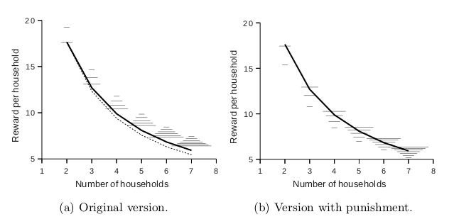
which uses a coalition of all N players (households). We use this to determine the optimal value of Pstart achievable by a memoryless strategy for each player, which we will then fix. These results are shown by the bold lines in the graphs below, where we vary the total number of households N. We also plot (as a dotted line) the values obtained if no demand-side management is applied.
Next, we consider the situation where a set of households C is allowed to deviate from the pre-agreed strategy, by choosing to ignore the limit clim if they wish. We check the same rPATL query as above, but using varying coalitions C of sizes from 1 to N. For the model of 3 households the following rPATL queries were used:
<<p1>> R{"value1"}max=? [F time=max_time]
<<p1,p2>> R{"value12"}max=? [F time=max_time]
<<p1,p2,p3>> R{"value123"}max=? [F time=max_time]
The resulting values are also plotted in graph (a) above, shown as horizontal dashes of width proportional to |C|: the shortest dash represents individual deviation, the longest is a collaboration of all households. The former shows the maximum value that can be achieved by following the optimal collaborative strategy, and in itself presents a benchmark for the performance of the original algorithm. The key result is that deviations by individuals or small coalitions guarantee a better expected value for the households than any larger collaboration: a highly undesired weakness for an MDSM system.
We propose a simple punishment mechanism that addresses the problem: we allow the distribution manager to cancel one job per step if the cost exceeds clim. The intuition is that, if a household is constantly abusing the system, its job could be cancelled. The code for the modified scheduler module is shown below.
// Model implementing demand-side energy management algorithm of:
// H. Hildmann and F. Saffre. Influence of Variable Supply and Load Flexibility on Demand-Side Management
// IEEE 8th International Conference on the European Energy Market (EEM). 2011.
//
// In contrast with original (DTMC) model, some agents are allowed to
// make a decision whether to execute their jobs modeled by non-determinism.
//
// Model has to be built using PRISM preprocessor (http://www.prismmodelchecker.org/prismpp/)
// using the following command: prismpp dsm_mdp-dtmc.pp <N> <D> <d> <L> <PS> > dsm_mdp-dtmc.pm, where
//
// <N> - number of households
// <D> - number of days
// <d> - number of deterministic households
// <L> - maximum job duration
// <PS> - 0.Pstart
//
//
// Aistis Simaitis 25/08/11


smg

// number of households
const int N = 3;

// number of days
const int D = 3;

// number of time intervals in the day
const int K = 16;

// expected number of jobs per household per day
const int Exp_J = 9;

// cost limits for households
const double price_limit = 1.5;

// initiation probabilities for jobs (uniform distribution)
const double P_J1 = 1/4;
const double P_J2 = 1/4;
const double P_J3 = 1/4;
const double P_J4 = 1/4;

// probability of starting a task independently of the cost
const double P_start = 0.8;

// distribution of the expected demand across intervals
const double D_K1 = 0.0614;
const double D_K2 = 0.0392;
const double D_K3 = 0.0304;
const double D_K4 = 0.0304;
const double D_K5 = 0.0355;
const double D_K6 = 0.0518;
const double D_K7 = 0.0651;
const double D_K8 = 0.0643;
const double D_K9 = 0.0625;
const double D_K10 = 0.0618;
const double D_K11 = 0.0614;
const double D_K12 = 0.0695;
const double D_K13 = 0.0887;
const double D_K14 = 0.1013;
const double D_K15 = 0.1005;
const double D_K16 = 0.0762;

// time limit
const int max_time = K*D+1;

// ---------------------------------------------------

// time counter
global time : [1..max_time];

// jobs of households
global job1 : [0..4];
global job2 : [0..4];
global job3 : [0..4];

// scheduling variable
global sched : [0..N];


player p0
 	player0
endplayer

// definition of scheduling module
module player0

// cost is below the limit
	[] sched = 0 -> 1/N : (sched'=1)
		      + 1/N : (sched'=2)
		      + 1/N : (sched'=3)
;

// cost is above the limit - allowing scheduler to switch off one job
	[] sched = 0 & jobs_running > price_limit & job1>0 -> 1/N : (sched'=1) & (job1'=0)
		      					      + 1/N : (sched'=2) & (job1'=0)
		      					      + 1/N : (sched'=3) & (job1'=0)
;
	[] sched = 0 & jobs_running > price_limit & job2>0 -> 1/N : (sched'=1) & (job2'=0)
		      					      + 1/N : (sched'=2) & (job2'=0)
		      					      + 1/N : (sched'=3) & (job2'=0)
;
	[] sched = 0 & jobs_running > price_limit & job3>0 -> 1/N : (sched'=1) & (job3'=0)
		      					      + 1/N : (sched'=2) & (job3'=0)
		      					      + 1/N : (sched'=3) & (job3'=0)
;

endmodule


// definitions of non-deterministic households
player p1
	player1, [start1], [backoff1], [nbackoff1]
endplayer

module player1

	job_arrived1 : [0..4];

	[] sched=1 & active = 0 & job1 > 0 & time < max_time -> (job1'=new_j1) & (job2'=new_j2) & (job3'=new_j3) & (time'=time+1) & (sched'=0);

	// initiate the job with probability P_init
	[] sched=1 & active = 0 & job1 = 0 & time < max_time -> P_init*P_J1 : (job_arrived1'=1)
							    + P_init*P_J2 : (job_arrived1'=2)
							    + P_init*P_J3 : (job_arrived1'=3)
							    + P_init*P_J4 : (job_arrived1'=4)
				       			    + (1-P_init) : (job1'=new_j1) & (job2'=new_j2) & (job3'=new_j3) & (time'=time+1) & (sched'=0);

	// start job if cost below the limit
	[start1] sched=1 & job_arrived1 > 0 & price <= price_limit & time < max_time-> (job1'=job_arrived1)  & (job2'=new_j2) & (job3'=new_j3) & (job_arrived1'=0) & (time'=time+1) & (sched'=0);

	// back-off with probability 1-P_start
	[backoff1] sched=1 & job_arrived1 > 0 & price > price_limit & time < max_time->   P_start : (job1'=job_arrived1)  & (job2'=new_j2) & (job3'=new_j3) & (job_arrived1'=0) & (time'=time+1) & (sched'=0)
						   + (1-P_start) : (job1'=new_j1) & (job2'=new_j2) & (job3'=new_j3) & (job_arrived1'=0) & (time'=time+1) & (sched'=0);

	// don't back-off
	[nbackoff1] sched=1 & job_arrived1 > 0 & price > price_limit & time < max_time -> (job1'=job_arrived1)  & (job2'=new_j2) & (job3'=new_j3) & (job_arrived1'=0) & (time'=time+1) & (sched'=0);

	// finished
	[] sched=1 & time=max_time -> (job1'=new_j1) & (job2'=new_j2) & (job3'=new_j3) & (sched'=0);

endmodule

player p2
	player2, [start2], [backoff2], [nbackoff2]
endplayer

module player2

	job_arrived2 : [0..4];

	[] sched=2 & active = 0 & job2 > 0 & time < max_time -> (job1'=new_j1) & (job2'=new_j2) & (job3'=new_j3) & (time'=time+1) & (sched'=0);

	// initiate the job with probability P_init
	[] sched=2 & active = 0 & job2 = 0 & time < max_time -> P_init*P_J1 : (job_arrived2'=1)
							    + P_init*P_J2 : (job_arrived2'=2)
							    + P_init*P_J3 : (job_arrived2'=3)
							    + P_init*P_J4 : (job_arrived2'=4)
				       			    + (1-P_init) : (job1'=new_j1) & (job2'=new_j2) & (job3'=new_j3) & (time'=time+1) & (sched'=0);

	// start job if cost below the limit
	[start2] sched=2 & job_arrived2 > 0 & price <= price_limit & time < max_time-> (job2'=job_arrived2)  & (job1'=new_j1) & (job3'=new_j3) & (job_arrived2'=0) & (time'=time+1) & (sched'=0);

	// back-off with probability 1-P_start
	[backoff2] sched=2 & job_arrived2 > 0 & price > price_limit & time < max_time->   P_start : (job2'=job_arrived2)  & (job1'=new_j1) & (job3'=new_j3) & (job_arrived2'=0) & (time'=time+1) & (sched'=0)
						   + (1-P_start) : (job1'=new_j1) & (job2'=new_j2) & (job3'=new_j3) & (job_arrived2'=0) & (time'=time+1) & (sched'=0);

	// don't back-off
	[nbackoff2] sched=2 & job_arrived2 > 0 & price > price_limit & time < max_time -> (job2'=job_arrived2)  & (job1'=new_j1) & (job3'=new_j3) & (job_arrived2'=0) & (time'=time+1) & (sched'=0);

	// finished
	[] sched=2 & time=max_time -> (job1'=new_j1) & (job2'=new_j2) & (job3'=new_j3) & (sched'=0);

endmodule

player p3
	player3, [start3], [backoff3], [nbackoff3]
endplayer

module player3

	job_arrived3 : [0..4];

	[] sched=3 & active = 0 & job3 > 0 & time < max_time -> (job1'=new_j1) & (job2'=new_j2) & (job3'=new_j3) & (time'=time+1) & (sched'=0);

	// initiate the job with probability P_init
	[] sched=3 & active = 0 & job3 = 0 & time < max_time -> P_init*P_J1 : (job_arrived3'=1)
							    + P_init*P_J2 : (job_arrived3'=2)
							    + P_init*P_J3 : (job_arrived3'=3)
							    + P_init*P_J4 : (job_arrived3'=4)
				       			    + (1-P_init) : (job1'=new_j1) & (job2'=new_j2) & (job3'=new_j3) & (time'=time+1) & (sched'=0);

	// start job if cost below the limit
	[start3] sched=3 & job_arrived3 > 0 & price <= price_limit & time < max_time-> (job3'=job_arrived3)  & (job1'=new_j1) & (job2'=new_j2) & (job_arrived3'=0) & (time'=time+1) & (sched'=0);

	// back-off with probability 1-P_start
	[backoff3] sched=3 & job_arrived3 > 0 & price > price_limit & time < max_time->   P_start : (job3'=job_arrived3)  & (job1'=new_j1) & (job2'=new_j2) & (job_arrived3'=0) & (time'=time+1) & (sched'=0)
						   + (1-P_start) : (job1'=new_j1) & (job2'=new_j2) & (job3'=new_j3) & (job_arrived3'=0) & (time'=time+1) & (sched'=0);

	// don't back-off
	[nbackoff3] sched=3 & job_arrived3 > 0 & price > price_limit & time < max_time -> (job3'=job_arrived3)  & (job1'=new_j1) & (job2'=new_j2) & (job_arrived3'=0) & (time'=time+1) & (sched'=0);

	// finished
	[] sched=3 & time=max_time -> (job1'=new_j1) & (job2'=new_j2) & (job3'=new_j3) & (sched'=0);

endmodule


// definitions of deterministic households


// probability to initiate the load
formula P_init = Exp_J *
		 (mod(time,K) = 1 ? D_K1 :
		 (mod(time,K) = 2 ? D_K2 :
		 (mod(time,K) = 3 ? D_K3 :
		 (mod(time,K) = 4 ? D_K4 :
		 (mod(time,K) = 5 ? D_K5 :
		 (mod(time,K) = 6 ? D_K6 :
		 (mod(time,K) = 7 ? D_K7 :
		 (mod(time,K) = 8 ? D_K8 :
		 (mod(time,K) = 9 ? D_K9 :
		 (mod(time,K) = 10 ? D_K10 :
		 (mod(time,K) = 11 ? D_K11 :
		 (mod(time,K) = 12 ? D_K12 :
		 (mod(time,K) = 13 ? D_K13 :
		 (mod(time,K) = 14 ? D_K14 :
		 (mod(time,K) = 15 ? D_K15 :
		 D_K16)))))))))))))));

// formula to compute current cost
formula jobs_running = (job1>0?1:0)  + (job2>0?1:0) + (job3>0?1:0);

// formula to identify say that only one agent is active
formula active = job_arrived1 + job_arrived2  + job_arrived3 ;

// formula to update job status
formula new_j1 = job1=0?0:job1-1;
formula new_j2 = job2=0?0:job2-1;
formula new_j3 = job3=0?0:job3-1;

formula price = jobs_running+1;


rewards "cost"
	sched!=0 : jobs_running*jobs_running;
endrewards

rewards "tasks_started"
	sched!=0 & job1=1 : 1;
	sched!=0 & job2=1 : 1;
	sched!=0 & job3=1 : 1;
endrewards


rewards "value1"
	sched!=0 & job1>0 : 1/jobs_running;
endrewards
rewards "value12"
	sched!=0 & (job1>0|job2>0) : 1/jobs_running;
endrewards
rewards "value123"
	sched!=0 & (job1>0|job2>0|job3>0) : 1/jobs_running;
endrewards

rewards "value2"
	sched!=0 & job2>0 : 1/jobs_running;
endrewards
rewards "value3"
	sched!=0 & job3>0 : 1/jobs_running;
endrewards


rewards "common_value"
	sched!=0 : jobs_running=0?0:1/jobs_running;
endrewards
The results are shown in graph (b) above. This modification inverts the incentives so that now, for the individual agent, it is better to cooperate. Furthermore, there is a risk of getting a considerably lower payoff if the individual deviation is exercised. The best option now is full collaboration and small coalitions who deviate cannot guarantee better expected values any more.
Finally, we show, in the table below, some statistics for model size, construction time and time for model checking the property:
<<p1>> R{"value123"}max=? [F time=max_time]
The model checking was performed on a 2.80GHz PC with 32Gb of RAM.
| N: | Model: | Model checking: | ||||
| States: | Transitions: | Construction (s): | Property (s): | |||
| 2 | 5,302 | 8,328 | 0.585 | 0.349 | ||
| 3 | 33,528 | 82,560 | 1.062 | 3.0 | ||
| 4 | 178,272 | 473,088 | 2.898 | 16.562 | ||
| 5 | 743,904 | 2,145,120 | 14.488 | 69.936 | ||
| 6 | 2,384,369 | 7,260,756 | 56.859 | 232.12 | ||
| 7 | 6,241,312 | 19,678,246 | 214.974 | 749.62 | ||