

(Bouyer, Fahrenberg, Larsen & Markey)
Related publications: [NPS13] [KNP19]
One common use of (non-probabilistic) timed automata is the formalisation and solution of scheduler optimisation problems. In this case study, we consider an extension of the task-graph scheduling problem described in [BFLM11]. We show how probabilistic timed automata (PTAs) can be used to introduce uncertainty with regards to time delays and to consider the possibility of failures. We demonstrate how the digital clocks method can determine optimal schedulers for these problems, in terms of the (expected) time and energy consumption required to complete all tasks. We also use stochastic game variants of the models.
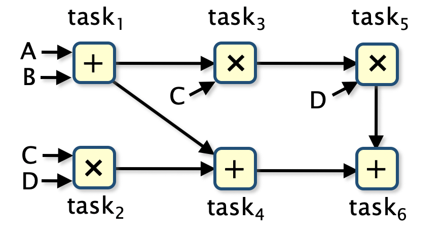
The basic model concerns computing the arithmetic expression D × (C × (A + B)) + ((A + B) + (C × D)) using two processors (P1 and P2) that have different speed and energy requirements. The specification of the processors is as follows.
| P1 | P2 | ||
| + | 2 picoseconds | 5 picoseconds | |
| × | 3 picoseconds | 7 picoseconds | |
| idle | 10 Watts | 20 Watts | |
| active | 90 Watts | 30 Watts |
The following figure presents a task graph for computing this expression and shows both the tasks that need to be performed (the subterms of the expression) and the dependencies between the tasks (the order the tasks must be evaluated in).
The system is formed as the parallel composition of three PTAs (PRISM modules), one for the scheduler and one for each processor is presented below.
// basic task graph model from
// Bouyer, Fahrenberg, Larsen and Markey
// Quantitative analysis of real-time systems using priced timed automata
// Communications of the ACM, 54(9):78–87, 2011

pta // model is a PTA

module scheduler

	task1 : [0..3]; // A+B
	task2 : [0..3]; // CxD
	task3 : [0..3]; // Cx(A+B)
	task4 : [0..3]; // (A+B)+(CxD)
	task5 : [0..3]; // DxCx(A+B)
	task6 : [0..3]; // (DxCx(A+B)) + ((A+B)+(CxD))

	// task status:
	// 0 - not started
	// 1 - running on processor 1
	// 2 - running on processor 2
	// 3 - task complete

	// start task 1
	[p1_add] task1=0 -> (task1'=1);
	[p2_add] task1=0 -> (task1'=2);

	// start task 2
	[p1_mult] task2=0 -> (task2'=1);
	[p2_mult] task2=0 -> (task2'=2);

	// start task 3 (must wait for task 1 to complete)
	[p1_mult] task3=0 & task1=3 -> (task3'=1);
	[p2_mult] task3=0 & task1=3 -> (task3'=2);

	// start task 4 (must wait for tasks 1 and 2 to complete)
	[p1_add] task4=0 & task1=3 & task2=3 -> (task4'=1);
	[p2_add] task4=0 & task1=3 & task2=3 -> (task4'=2);

	// start task 5 (must wait for task 3 to complete)
	[p1_mult] task5=0 & task3=3 -> (task5'=1);
	[p2_mult] task5=0 & task3=3 -> (task5'=2);

	// start task 6 (must wait for tasks 4 and 5 to complete)
	[p1_add] task6=0 & task4=3 & task5=3 -> (task6'=1);
	[p2_add] task6=0 & task4=3 & task5=3 -> (task6'=2);

	// a task finishes on processor 1
	[p1_done] task1=1 -> (task1'=3);
	[p1_done] task2=1 -> (task2'=3);
	[p1_done] task3=1 -> (task3'=3);
	[p1_done] task4=1 -> (task4'=3);
	[p1_done] task5=1 -> (task5'=3);
	[p1_done] task6=1 -> (task6'=3);

	// a task finishes on processor 2
	[p2_done] task1=2 -> (task1'=3);
	[p2_done] task2=2 -> (task2'=3);
	[p2_done] task3=2 -> (task3'=3);
	[p2_done] task4=2 -> (task4'=3);
	[p2_done] task5=2 -> (task5'=3);
	[p2_done] task6=2 -> (task6'=3);

endmodule

// processor 1
module P1

	p1 : [0..2];
	// 0 - idle
	// 1 - add
	// 2 - multiply

	x1 : clock; // local clock

	invariant
        (p1=1 => x1<=2) &
        (p1=2 => x1<=3)
    endinvariant

	// addition
	[p1_add] p1=0 -> (p1'=1) & (x1'=0); // start
	[p1_done] p1=1 & x1=2 -> (p1'=0) & (x1'=0); // finish

	// multiplication
	[p1_mult] p1=0 -> (p1'=2) & (x1'=0); // start
	[p1_done] p1=2 & x1=3 -> (p1'=0) & (x1'=0);  // finish

endmodule

// processor 2
module P2

	p2 : [0..2];
	// 0 - idle
	// 1 - add
	// 2 - multiply

	x2 : clock; // local clock

	invariant
        (p2=1 => x2<=5) &
        (p2=2 => x2<=7)
    endinvariant

	// addition
	[p2_add] p2=0 -> (p2'=1) & (x2'=0); // start
	[p2_done] p2=1 & x2=5 -> (p2'=0) & (x2'=0); // finish

	// multiplication
	[p2_mult] p2=0 -> (p2'=2) & (x2'=0); // start
	[p2_done] p2=2 & x2=7 -> (p2'=0) & (x2'=0);  // finish

endmodule

// reward structure: elapsed time
rewards "time"
	true : 1;
endrewards

// reward structures: energy consumption
rewards "energy"
	p1=0 : 10/1000;
	p1>0 : 90/1000;
	p2=0 : 20/1000;
	p2>0 : 30/1000;
endrewards

// target state (all tasks complete)
label "tasks_complete" = (task6=3);
The actions p1_add and p1_mult represent an addition and multiplication task being scheduled on P1 respectively, while the action p1_done indicates that the current task has been completed on P1. There are similar actions for P2. The systems includes clocks x1 and x2 which is used to keep track of the time that a task has been running on P1 and P2 respectively, and are therefore reset when a task starts and the invariants and guards correspond to the time required to complete the tasks of addition and multiplication on the processors.
We consider the following properties of the system.
// scheduler can complete all tasks (max probability all tasks complete equals 1)
Pmax=?[F "tasks_complete" ];

// min expected time to complete all tasks
R{"time"}min=?[F "tasks_complete" ];

// min expected energy to complete all tasks
R{"energy"}min=?[F "tasks_complete" ];
Using the digital clocks PTA engine we find the following optimal scheduler for minimising the elapsed time to complete all tasks, which takes 12 picoseconds to complete all tasks.
| time | 1 | 2 | 3 | 4 | 5 | 6 | 7 | 8 | 9 | 10 | 11 | 12 | 13 | 14 | 15 | 16 | 17 | 18 | 19 | 20 | |
| P1 | task1 | task3 | task5 | task4 | task6 | ||||||||||||||||
| P2 | task2 | ||||||||||||||||||||
In the case of energy consumption, we find an optimal scheduler which requires 1.3200 nanojoules and schedules tasks as shown below.
| time | 1 | 2 | 3 | 4 | 5 | 6 | 7 | 8 | 9 | 10 | 11 | 12 | 13 | 14 | 15 | 16 | 17 | 18 | 19 | 20 | |
| P1 | task1 | task3 | task4 | ||||||||||||||||||
| P2 | task2 | task5 | task6 | ||||||||||||||||||
We now extend the basic model making the time required for each processor to perform a task probabilistic. More precisely, if, in the original problem the time for a processor to perform a task was k, we suppose now that the time taken is uniformly distributed between the delays k-1, k and k+1.
The PRISM model for this scenario is presented below. Note that to prevent the scheduler from seeing into the future when making decisions, the probabilistic choice for task completion is made on completion rather than on initialisation.
// task graph model with random execution times
// extends the task graph problem from
// Bouyer, Fahrenberg, Larsen and Markey
// Quantitative analysis of real-time systems using priced timed automata
// Communications of the ACM, 54(9):78–87, 2011

pta // model is a PTA

module scheduler

	task1 : [0..3]; // A+B
	task2 : [0..3]; // CxD
	task3 : [0..3]; // Cx(A+B)
	task4 : [0..3]; // (A+B)+(CxD)
	task5 : [0..3]; // DxCx(A+B)
	task6 : [0..3]; // (DxCx(A+B)) + ((A+B)+(CxD))

	// task status:
	// 0 - not started
	// 1 - running on processor 1
	// 2 - running on processor 2
	// 3 - task complete

	// start task 1
	[p1_add] task1=0 -> (task1'=1);
	[p2_add] task1=0 -> (task1'=2);

	// start task 2
	[p1_mult] task2=0 -> (task2'=1);
	[p2_mult] task2=0 -> (task2'=2);

	// start task 3 (must wait for task 1 to complete)
	[p1_mult] task3=0 & task1=3 -> (task3'=1);
	[p2_mult] task3=0 & task1=3 -> (task3'=2);

	// start task 4 (must wait for tasks 1 and 2 to complete)
	[p1_add] task4=0 & task1=3 & task2=3 -> (task4'=1);
	[p2_add] task4=0 & task1=3 & task2=3 -> (task4'=2);

	// start task 5 (must wait for task 3 to complete)
	[p1_mult] task5=0 & task3=3 -> (task5'=1);
	[p2_mult] task5=0 & task3=3 -> (task5'=2);

	// start task 6 (must wait for tasks 4 and 5 to complete)
	[p1_add] task6=0 & task4=3 & task5=3 -> (task6'=1);
	[p2_add] task6=0 & task4=3 & task5=3 -> (task6'=2);

	// a task finishes on processor 1
	[p1_done] task1=1 -> (task1'=3);
	[p1_done] task2=1 -> (task2'=3);
	[p1_done] task3=1 -> (task3'=3);
	[p1_done] task4=1 -> (task4'=3);
	[p1_done] task5=1 -> (task5'=3);
	[p1_done] task6=1 -> (task6'=3);

	// a task finishes on processor 2
	[p2_done] task1=2 -> (task1'=3);
	[p2_done] task2=2 -> (task2'=3);
	[p2_done] task3=2 -> (task3'=3);
	[p2_done] task4=2 -> (task4'=3);
	[p2_done] task5=2 -> (task5'=3);
	[p2_done] task6=2 -> (task6'=3);

endmodule

// processor 1
module P1

	p1 : [0..3]; // 0 inactive, 1 - adding, 2 - multiplying, 3 - done
	c1 : [0..2]; // used for the uniform probabilistic choice of execution time
	x1 : clock; // local clock

	invariant
        (p1=1 => x1<=1) &
        ((p1=2 & c1=0) => x1<=2) &
        ((p1=2 & c1>0)=> x1<=1) &
        (p1=3 => x1<=0)
    endinvariant

	// addition
	[p1_add] p1=0 -> (p1'=1) & (x1'=0); // start
	[] p1=1 & x1=1 & c1=0 -> 1/3 : (p1'=3) & (x1'=0) & (c1'=0)
	                             + 2/3 : (c1'=1) & (x1'=0); // k-1
	[] p1=1 & x1=1 & c1=1 -> 1/2 : (p1'=3) & (x1'=0) & (c1'=0)
	                             + 1/2 : (c1'=2) & (x1'=0); // k
	[p1_done] p1=1 & x1=1 & c1=2 -> (p1'=0) & (x1'=0) & (c1'=0); // k+1

	// multiplication
	[p1_mult] p1=0 -> (p1'=2) & (x1'=0); // start
	[] p1=2 & x1=2 & c1=0 -> 1/3 : (p1'=3) & (x1'=0) & (c1'=0)
	                             + 2/3 : (c1'=1) & (x1'=0); // k-1
	[] p1=2 & x1=1 & c1=1 -> 1/2 : (p1'=3) & (x1'=0) & (c1'=0)
	                             + 1/2 : (c1'=2) & (x1'=0); // k
	[p1_done] p1=2 & x1=1 & c1=2 -> (p1'=0) & (x1'=0) & (c1'=0); // k+1

	[p1_done] p1=3 -> (p1'=0);  // finish

endmodule

// processor 2
module P2

	p2 : [0..3]; // 0 inactive, 1 - adding, 2 - multiplying, 3 - done
	c2 : [0..2]; // used for the uniform probabilistic choice of execution time
	x2 : clock; // local clock

	invariant
        ((p2=1 & c2=0) => x2<=4) &
        ((p2=1 & c2>0)=> x2<=1) &
        ((p2=2 & c2=0) => x2<=6) &
        ((p2=2 & c2>0)=> x2<=1) &
        (p2=3 => x2<=0)
    endinvariant

	// addition
	[p2_add] p2=0 -> (p2'=1) & (x2'=0); // start
	[] p2=1 & x2=4 & c2=0 -> 1/3 : (p2'=3) & (x2'=0) & (c2'=0)
	                             + 2/3 : (c2'=1) & (x2'=0); // k-1
	[] p2=1 & x2=1 & c2=1 -> 1/2 : (p2'=3) & (x2'=0) & (c2'=0)
	                             + 1/2 : (c2'=2) & (x2'=0); // k
	[p2_done] p2=1 & x2=1 & c2=2 -> (p2'=0) & (x2'=0) & (c2'=0); // k+1

	// multiplication
	[p2_mult] p2=0 -> (p2'=2) & (x2'=0); // start
	[] p2=2 & x2=6 & c2=0 -> 1/3 : (p2'=3) & (x2'=0) & (c2'=0)
	                             + 2/3 : (c2'=1) & (x2'=0); // k-1
	[] p2=2 & x2=1 & c2=1 -> 1/2 : (p2'=3) & (x2'=0) & (c2'=0)
	                             + 1/2 : (c2'=2) & (x2'=0); // k
	[p2_done] p2=2 & x2=1 & c2=2 -> (p2'=0) & (x2'=0) & (c2'=0); // k+1
	[p2_done] p2=3 -> (p2'=0);  // finish

endmodule

// reward structure: elapsed time
rewards "time"
	true : 1;
endrewards

// reward structures: energy consumption
rewards "energy"
	p1=0 : 10/1000;
	p1>0 : 90/1000;
	p2=0 : 20/1000;
	p2>0 : 30/1000;
endrewards

// target state (all tasks complete)
label "tasks_complete" = (task6=3);
Analysing this model, we find that the optimal expected time and energy consumption to complete all tasks equal 12.226 picoseconds and 1.3201 nanojoules, respectively. This improves on the results obtained using the optimal schedulers for the original model, where the expected time and energy consumption equal 13.1852 picoseconds and 1.3211 nanojoules, respectively.
Synthesising optimal schedulers, we find that they change their decision based upon the delays of previously completed tasks. For example, for elapsed time, the optimal scheduler starts as for the non-probabilistic case, first scheduling task1 followed by task3 on P1 and task2 on P2. However, it is now possible for task2 to complete before task3 (if the execution times for task1, task2 and task3 are 3, 6 and 4 picoseconds respectively), in which case the optimal scheduler now makes a different decision from the non-probabilistic case. Under one possible set of execution times for the remaining tasks, the optimal scheduling is as follows:
| time | 1 | 2 | 3 | 4 | 5 | 6 | 7 | 8 | 9 | 10 | 11 | 12 | 13 | 14 | 15 | 16 | 17 | 18 | 19 | 20 | |
| P1 | task1 | task3 | task5 | task6 | |||||||||||||||||
| P2 | task2 | task4 | |||||||||||||||||||
As a second extension of the scheduling problem, we add a third processor P3 which consumes the same energy as P2 but is faster (addition takes 3 picoseconds and multiplication 5 picoseconds). However, this comes at a cost: there is a chance (probability p) that the processor fails and the computation must be rescheduled and performed again.
The PRISM model for this scenario is presented below. Note that to prevent the scheduler from seeing into the future when making decisions, the probabilistic choice for task completion is made on completion rather than on initialisation.
// basic task graph model from
// Bouyer, Fahrenberg, Larsen and Markey
// Quantitative analysis of real-time systems using priced timed automata
// Communications of the ACM, 54(9):78–87, 2011

pta // model is a PTA

// probability P3 fails
const double p;

module scheduler

	task1 : [0..4]; // A+B
	task2 : [0..4]; // CxD
	task3 : [0..4]; // Cx(A+B)
	task4 : [0..4]; // (A+B)+(CxD)
	task5 : [0..4]; // DxCx(A+B)
	task6 : [0..4]; // (DxCx(A+B)) + ((A+B)+(CxD))

	// task status:
	// 0 - not started
	// 1 - running on processor 1
	// 2 - running on processor 2
	// 3 - running on processor 3
	// 4 - task complete

	// start task 1
	[p1_add] task1=0 -> (task1'=1);
	[p2_add] task1=0 -> (task1'=2);
	[p3_add] task1=0 -> (task1'=3);

	// start task 2
	[p1_mult] task2=0 -> (task2'=1);
	[p2_mult] task2=0 -> (task2'=2);
	[p3_mult] task2=0 -> (task2'=3);

	// start task 3 (must wait for task 1 to complete)
	[p1_mult] task3=0 & task1=4 -> (task3'=1);
	[p2_mult] task3=0 & task1=4 -> (task3'=2);
	[p3_mult] task3=0 & task1=4 -> (task3'=3);

	// start task 4 (must wait for tasks 1 and 2 to complete)
	[p1_add] task4=0 & task1=4 & task2=4 -> (task4'=1);
	[p2_add] task4=0 & task1=4 & task2=4 -> (task4'=2);
	[p3_add] task4=0 & task1=4 & task2=4 -> (task4'=3);

	// start task 5 (must wait for task 3 to complete)
	[p1_mult] task5=0 & task3=4 -> (task5'=1);
	[p2_mult] task5=0 & task3=4 -> (task5'=2);
	[p3_mult] task5=0 & task3=4 -> (task5'=3);

	// start task 6 (must wait for tasks 4 and 5 to complete)
	[p1_add] task6=0 & task4=4 & task5=4 -> (task6'=1);
	[p2_add] task6=0 & task4=4 & task5=4 -> (task6'=2);
	[p3_add] task6=0 & task4=4 & task5=4 -> (task6'=3);

	// a task finishes on processor 1
	[p1_done] task1=1 -> (task1'=4);
	[p1_done] task2=1 -> (task2'=4);
	[p1_done] task3=1 -> (task3'=4);
	[p1_done] task4=1 -> (task4'=4);
	[p1_done] task5=1 -> (task5'=4);
	[p1_done] task6=1 -> (task6'=4);

	// a task finishes on processor 2
	[p2_done] task1=2 -> (task1'=4);
	[p2_done] task2=2 -> (task2'=4);
	[p2_done] task3=2 -> (task3'=4);
	[p2_done] task4=2 -> (task4'=4);
	[p2_done] task5=2 -> (task5'=4);
	[p2_done] task6=2 -> (task6'=4);

	// a task finishes on processor 2
	[p3_done] task1=3 -> (task1'=4);
	[p3_done] task2=3 -> (task2'=4);
	[p3_done] task3=3 -> (task3'=4);
	[p3_done] task4=3 -> (task4'=4);
	[p3_done] task5=3 -> (task5'=4);
	[p3_done] task6=3 -> (task6'=4);
	[p3_fail] task1=3 -> (task1'=0);
	[p3_fail] task2=3 -> (task2'=0);
	[p3_fail] task3=3 -> (task3'=0);
	[p3_fail] task4=3 -> (task4'=0);
	[p3_fail] task5=3 -> (task5'=0);
	[p3_fail] task6=3 -> (task6'=0);

endmodule

// processor 1
module P1

	p1 : [0..2];
	// 0 - idle
	// 1 - add
	// 2 - multiply

	x1 : clock; // local clock

	invariant
        (p1=1 => x1<=2) &
        (p1=2 => x1<=3)
    endinvariant

	// addition
	[p1_add] p1=0 -> (p1'=1) & (x1'=0); // start
	[p1_done] p1=1 & x1=2 -> (p1'=0) & (x1'=0); // finish

	// multiplication
	[p1_mult] p1=0 -> (p1'=2) & (x1'=0); // start
	[p1_done] p1=2 & x1=3 -> (p1'=0) & (x1'=0);  // finish

endmodule

// processor 2
module P2

	p2 : [0..2];
	// 0 - idle
	// 1 - add
	// 2 - multiply

	x2 : clock; // local clock

	invariant
        (p2=1 => x2<=5) &
        (p2=2 => x2<=7)
    endinvariant

	// addition
	[p2_add] p2=0 -> (p2'=1) & (x2'=0); // start
	[p2_done] p2=1 & x2=5 -> (p2'=0) & (x2'=0); // finish

	// multiplication
	[p2_mult] p2=0 -> (p2'=2) & (x2'=0); // start
	[p2_done] p2=2 & x2=7 -> (p2'=0) & (x2'=0);  // finish

endmodule

// processor 3 (faster than processor 2 but can fail)
module P3

	p3 : [0..3];
	// 0 - idle
	// 1 - add
	// 2 - multiply
	fail3 : [0..1]; // failed to complete task

	x3 : clock; // local clock

	invariant
        (p3=1 => x3<=3) &
        (p3=2 => x3<=5) &
        (p3=3 => x3<=0)
    endinvariant

	// addition
	[p3_add] p3=0 -> (p3'=1) & (x3'=0); // start
	[] p3=1 & x3=3 -> p : (fail3'=1) & (p3'=3) & (x3'=0)  // fail
	                + (1-p) : (fail3'=0) & (p3'=3) & (x3'=0); // finish

	// multiplication
	[p3_mult] p3=0 -> (p3'=2) & (x3'=0); // start
	[] p3=2 & x3=5 -> p : (fail3'=1) & (p3'=3) & (x3'=0) // fail
	                + (1-p) : (fail3'=0) & (p3'=3) & (x3'=0); // finish

	[p3_fail] p3=3 & fail3=1 -> (p3'=0) & (x3'=0) & (fail3'=0); // failed
	[p3_done] p3=3 & fail3=0 -> (p3'=0) & (x3'=0) & (fail3'=0); // completed

endmodule

// reward structure: elapsed time
rewards "time"
	true : 1;
endrewards

// reward structures: energy consumption
rewards "energy"
	p1=0 : 10/1000;
	p1>0 : 90/1000;
	p2=0 : 20/1000;
	p2>0 : 30/1000;
endrewards

// target state (all tasks complete)
label "tasks_complete" = (task6=4);
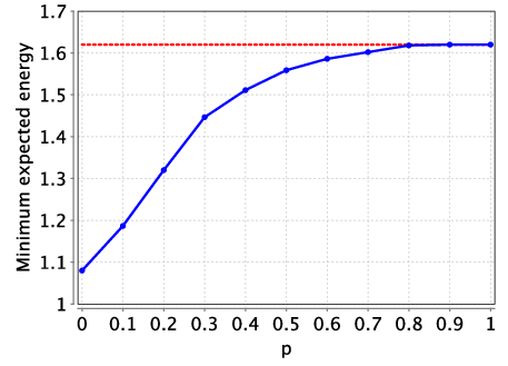
Analysing this model, we find that for small values of p (the probability of P3 failing to successfully complete a task), as P3 has better performance than P2, both the optimal expected time and energy consumption can be improved using P3. However, as the probability of failure increases, P3’s better performance is out-weighed by the chance of its failure and using it no longer yields optimal values. This can be seen in the following graphs which plot the optimal expected time and energy consumption for this extended model as the failure probability p varies.

For example, we give an optimal scheduler for the expected time when p=0.25 which takes 11.0625 picoseconds (the optimal expected time is 12 picoseconds when P3 is not used). The dark boxes are used to denote the cases when P3 is scheduled to complete a task, but experiences a fault and does not complete the scheduled task correctly.
| time | 1 | 2 | 3 | 4 | 5 | 6 | 7 | 8 | 9 | 10 | 11 | 12 | 13 | 14 | 15 | 16 | 17 | 18 | 19 | 20 | |
| P1 | task1 | task3 | task5 | task6 | |||||||||||||||||
| P2 | |||||||||||||||||||||
| P3 | task2 | task4 | |||||||||||||||||||
| time | 1 | 2 | 3 | 4 | 5 | 6 | 7 | 8 | 9 | 10 | 11 | 12 | 13 | 14 | 15 | 16 | 17 | 18 | 19 | 20 | |
| P1 | task1 | task3 | task2 | task5 | task6 | ||||||||||||||||
| P2 | |||||||||||||||||||||
| P3 | task2 | task4 | |||||||||||||||||||
| time | 1 | 2 | 3 | 4 | 5 | 6 | 7 | 8 | 9 | 10 | 11 | 12 | 13 | 14 | 15 | 16 | 17 | 18 | 19 | 20 | |
| P1 | task1 | task3 | task2 | task4 | task? | ||||||||||||||||
| P2 | |||||||||||||||||||||
| P3 | task2 | task4 | |||||||||||||||||||
| time | 1 | 2 | 3 | 4 | 5 | 6 | 7 | 8 | 9 | 10 | 11 | 12 | 13 | 14 | 15 | 16 | 17 | 18 | 19 | 20 | |
| P1 | task1 | task3 | task5 | task4 | task6 | ||||||||||||||||
| P2 | |||||||||||||||||||||
| P3 | task2 | task4 | |||||||||||||||||||
A limitation of the above models is that the execution time of the processors (or its probability distribution) must be known and remain fixed. We now remove this restriction by moving to a game-based model in which there are two players:
The model is a TPTG (turned-based probabilistic timed game) which is an extension of a PTA to incorporate multiple players by allocating locations to different players. TPTGs are specified in PRISM-games in a similar fashion to (discrete-time) turn-based stochastic games (SMGs), by assigning modules and actions to players. The locations under the control of a specific player correspond to those for which either an action or module with an unlabelled transition which is under the control of that player.
Below we give the TPTG model for the basic model.
// turn based probabilistic timed game model of the task graph from
// Bouyer, Fahrenberg, Larsen and Markey
// Quantitative analysis of real-time systems using priced timed automata
// Communications of the ACM, 54(9):78–87, 2011

tptg

// scheduler
player sched
  scheduler, [p1_add], [p2_add], [p1_mult], [p2_mult]
endplayer

// environment
player env
  P1, P2, [p1_done], [p2_done]
endplayer

module scheduler

	turn : [0..1]; 	// use to classify player 1 and player 2 states

	task1 : [0..3]; // A+B
	task2 : [0..3]; // CxD
	task3 : [0..3]; // Cx(A+B)
	task4 : [0..3]; // (A+B)+(CxD)
	task5 : [0..3]; // DxCx(A+B)
	task6 : [0..3]; // (DxCx(A+B)) + ((A+B)+(CxD))

	// task status:
	// 0 - not started
	// 1 - running on processor 1
	// 2 - running on processor 2
	// 3 - task complete

	y : clock; // local clock

	invariant
			// cannot let time pass if a task is scheduled
			// as must pass over control to the environment
			((turn=0 & ((p1>1 | p2>1)|(task6!=3))) => y<=0)
	endinvariant

	// finished scheduling and hand control over to the environment
	[] turn=0 -> (turn'=1);

	// start task 1
	[p1_add] turn=0 & task1=0 -> (task1'=1);
	[p2_add] turn=0 & task1=0 -> (task1'=2);

	// start task 2
	[p1_mult] turn=0 & task2=0 -> (task2'=1);
	[p2_mult] turn=0 & task2=0 -> (task2'=2);

	// start task 3 (must wait for task 1 to complete)
	[p1_mult] turn=0 & task3=0 & task1=3 -> (task3'=1);
	[p2_mult] turn=0 & task3=0 & task1=3 -> (task3'=2);

	// start task 4 (must wait for tasks 1 and 2 to complete)
	[p1_add] turn=0 & task4=0 & task1=3 & task2=3 -> (task4'=1);
	[p2_add] turn=0 & task4=0 & task1=3 & task2=3 -> (task4'=2);

	// start task 5 (must wait for task 3 to complete)
	[p1_mult] turn=0 & task5=0 & task3=3 -> (task5'=1);
	[p2_mult] turn=0 & task5=0 & task3=3 -> (task5'=2);

	// start task 6 (must wait for tasks 4 and 5 to complete)
	[p1_add] turn=0 & task6=0 & task4=3 & task5=3 -> (task6'=1);
	[p2_add] turn=0 & task6=0 & task4=3 & task5=3 -> (task6'=2);

	// a task finishes on processor 1
	// and the scheduler takes over control
	[p1_done] task1=1 -> (task1'=3) & (y'=0) & (turn'=0);
	[p1_done] task2=1 -> (task2'=3) & (y'=0) & (turn'=0);
	[p1_done] task3=1 -> (task3'=3) & (y'=0) & (turn'=0);
	[p1_done] task4=1 -> (task4'=3) & (y'=0) & (turn'=0);
	[p1_done] task5=1 -> (task5'=3) & (y'=0) & (turn'=0);
	[p1_done] task6=1 -> (task6'=3) & (y'=0) & (turn'=0);

	// a task finishes on processor 2
	// and the scheduler takes over control
	[p2_done] task1=2 -> (task1'=3) & (y'=0) & (turn'=0);
	[p2_done] task2=2 -> (task2'=3) & (y'=0) & (turn'=0);
	[p2_done] task3=2 -> (task3'=3) & (y'=0) & (turn'=0);
	[p2_done] task4=2 -> (task4'=3) & (y'=0) & (turn'=0);
	[p2_done] task5=2 -> (task5'=3) & (y'=0) & (turn'=0);
	[p2_done] task6=2 -> (task6'=3) & (y'=0) & (turn'=0);

endmodule

// processor 1
module P1

	p1 : [0..2];
	// 0 - idle
	// 1 - add
	// 2 - multiply

	x1 : clock; // local clock

	invariant
			(p1=1 => x1<=2) &
			(p1=2 => x1<=3)
	endinvariant

	// addition
	[p1_add] p1=0 -> (p1'=1) & (x1'=0); // start
	[p1_done] turn=1 & p1=1 & x1<=2 -> (p1'=0) & (x1'=0); // finish

	// multiplication
	[p1_mult] p1=0 -> (p1'=2) & (x1'=0); // start
	[p1_done] turn=1 & p1=2 & x1<=3 -> (p1'=0) & (x1'=0);  // finish

endmodule

// processor 2
module P2

	p2 : [0..2];
	// 0 - idle
	// 1 - add
	// 2 - multiply

	x2 : clock; // local clock

	invariant
		(p2=1 => x2<=5) &
		(p2=2 => x2<=7)
	endinvariant

	// addition
	[p2_add] p2=0 -> (p2'=1) & (x2'=0); // start
	[p2_done] turn=1 & p2=1 & x2<=5 -> (p2'=0) & (x2'=0); // finish

	// multiplication
	[p2_mult] p2=0 -> (p2'=2) & (x2'=0); // start
	[p2_done] turn=1 & p2=2 & x2<=7 -> (p2'=0) & (x2'=0);  // finish

endmodule

// reward structure: elapsed time
rewards "time"
	true : 1;
endrewards

// reward structures: energy consumption
rewards "energy"
	p1=0 : 10/1000;
	p1>0 : 90/1000;
	p2=0 : 20/1000;
	p2>0 : 30/1000;
endrewards

// target state (all tasks complete)
label "tasks_complete" = (task6=3);
In the above model we use the turn variable to specify which locations are under the control of which player. When turn=0 the scheduler has control and when turn=1 the environment has control. Since the time taken for tasks to run is under the control of the environment, once tasks have been scheduled on time can pass until the scheduler has passed over control to the enronment, i.e. turn=1.
Using this model we can then ask which is the minimum execution time or energy consumption that the scheduler can ensure no matter how the environment behaves. In addition, we can find these minimum values when the players collaborate.
// min expected time to complete all tasks the scheduler can ensure
<<sched>>R{"time"}min=?[ F "tasks_complete" ];

// min expected energy to complete all tasks the scheduler can ensure
<<sched>>R{"energy"}min=?[ F "tasks_complete" ];

// min expected time to complete all tasks when players collaborate
<<sched,env>>R{"time"}min=?[ F "tasks_complete" ];

// min expected energy to complete all tasks when players collaborate
<<sched,env>>R{"energy"}min=?[ F "tasks_complete" ];
We find that the minimum values that the scheduler can ensure is the same as for the PTA model above, which demonstrates that in the worst case the environment delays tasks for as long as possible and the scheduler's optimal choices in this scenario is to follow the schedules given above for the PTA model.
As explained in [BFLM11], an optimal schedule for a game model in which delays can vary does not yield a simple assignment of tasks to processors at specific times as presented above for PTAs, but instead it is an assignment that also has as input when previous tasks were completed and on which processors.
We now extend the basic TPTG model by allowing the processors P1 and P2 to have at most k1 and k2 faults respectively. We assume that the probability of any fault causing a failure is p and faults can happen at any time a processor is active, i.e., the time the faults occur is under the control of the environment. Again, we could not model this extension with a PTA, since the scheduler would then be in control of when the faults occurred, and therefore in the optimal case would decide that no faults would occur.
// turn based probabilistic timed game model of the task graph from
// Bouyer, Fahrenberg, Larsen and Markey
// Quantitative analysis of real-time systems using priced timed automata
// Communications of the ACM, 54(9):78–87, 2011
// extended to allow processors to have faults that probabilistically cause failures

tptg

// scheduler
player sched
  scheduler, [p1_add], [p2_add], [p1_mult], [p2_mult]
endplayer

// environment
player env
  P1, P2, [p1_done], [p2_done], [p1_fail], [p2_fail]
endplayer

const int k1; // number of possible faults for processor 1
const int k2; // number of possible faults for processor 2
const double p; // probability fault causes a failure

module scheduler

	turn : [0..1]; 	// use to classify player 1 and player 2 states

	task1 : [0..3]; // A+B
	task2 : [0..3]; // CxD
	task3 : [0..3]; // Cx(A+B)
	task4 : [0..3]; // (A+B)+(CxD)
	task5 : [0..3]; // DxCx(A+B)
	task6 : [0..3]; // (DxCx(A+B)) + ((A+B)+(CxD))

	// task status:
	// 0 - not started
	// 1 - running on processor 1
	// 2 - running on processor 2
	// 3 - task complete

	y : clock; // local clock

	invariant
			// cannot let time pass if a task is scheduled
			// as must pass over control to the environment
			((turn=0 & ((p1>1 | p2>1)|(task6!=3))) => y<=0)
	endinvariant

	// finished scheduling and hand control over to the environment
	[] turn=0 -> (turn'=1);

	// start task 1
	[p1_add] turn=0 & task1=0 -> (task1'=1);
	[p2_add] turn=0 & task1=0 -> (task1'=2);

	// start task 2
	[p1_mult] turn=0 & task2=0 -> (task2'=1);
	[p2_mult] turn=0 & task2=0 -> (task2'=2);

	// start task 3 (must wait for task 1 to complete)
	[p1_mult] turn=0 & task3=0 & task1=3 -> (task3'=1);
	[p2_mult] turn=0 & task3=0 & task1=3 -> (task3'=2);

	// start task 4 (must wait for tasks 1 and 2 to complete)
	[p1_add] turn=0 & task4=0 & task1=3 & task2=3 -> (task4'=1);
	[p2_add] turn=0 & task4=0 & task1=3 & task2=3 -> (task4'=2);

	// start task 5 (must wait for task 3 to complete)
	[p1_mult] turn=0 & task5=0 & task3=3 -> (task5'=1);
	[p2_mult] turn=0 & task5=0 & task3=3 -> (task5'=2);

	// start task 6 (must wait for tasks 4 and 5 to complete)
	[p1_add] turn=0 & task6=0 & task4=3 & task5=3 -> (task6'=1);
	[p2_add] turn=0 & task6=0 & task4=3 & task5=3 -> (task6'=2);

	// a task finishes on processor 1
	[p1_done] task1=1 -> (task1'=3) & (y'=0) & (turn'=0);
	[p1_done] task2=1 -> (task2'=3) & (y'=0) & (turn'=0);
	[p1_done] task3=1 -> (task3'=3) & (y'=0) & (turn'=0);
	[p1_done] task4=1 -> (task4'=3) & (y'=0) & (turn'=0);
	[p1_done] task5=1 -> (task5'=3) & (y'=0) & (turn'=0);
	[p1_done] task6=1 -> (task6'=3) & (y'=0) & (turn'=0);

	// a task finishes on processor 2
	[p2_done] task1=2 -> (task1'=3) & (y'=0) & (turn'=0);
	[p2_done] task2=2 -> (task2'=3) & (y'=0) & (turn'=0);
	[p2_done] task3=2 -> (task3'=3) & (y'=0) & (turn'=0);
	[p2_done] task4=2 -> (task4'=3) & (y'=0) & (turn'=0);
	[p2_done] task5=2 -> (task5'=3) & (y'=0) & (turn'=0);
	[p2_done] task6=2 -> (task6'=3) & (y'=0) & (turn'=0);

	// a task fails on processor 1
	[p1_fail] task1=1 -> (task1'=0) & (turn'=0);
	[p1_fail] task2=1 -> (task2'=0) & (turn'=0);
	[p1_fail] task3=1 -> (task3'=0) & (turn'=0);
	[p1_fail] task4=1 -> (task4'=0) & (turn'=0);
	[p1_fail] task5=1 -> (task5'=0) & (turn'=0);
	[p1_fail] task6=1 -> (task6'=0) & (turn'=0);

	// a task fails on processor 2
	[p2_fail] task1=2 -> (task1'=0) & (turn'=0);
	[p2_fail] task2=2 -> (task2'=0) & (turn'=0);
	[p2_fail] task3=2 -> (task3'=0) & (turn'=0);
	[p2_fail] task4=2 -> (task4'=0) & (turn'=0);
	[p2_fail] task5=2 -> (task5'=0) & (turn'=0);
	[p2_fail] task6=2 -> (task6'=0) & (turn'=0);

endmodule

// processor 1
module P1

	p1 : [0..2];
	// 0 - idle
	// 1 - add
	// 2 - multiply
	fail1 : [0..k2+1]; // number of failures

	x1 : clock; // local clock

	invariant
			(p1=1 => x1<=2) &
			(p1=2 => x1<=3) &
			(p1=3 => x1<=0) &
			(p1=4 => x1<=0)
	endinvariant

	// addition
	[p1_add] p1=0 -> (p1'=1) & (x1'=0); // start
	[p1_done] turn=1 & (p1=1) & (x1<=2) -> (p1'=0) & (x1'=0); // finish
	[] turn=1 & (p1=1) & (x1<=2) & (fail1<k1) -> p : (fail1'=fail1+1) & (p1'=3) & (x1'=0)
											 + 1-p : (fail1'=fail1+1) & (p1'=1); // fault
	// multiplication
	[p1_mult] p1=0 -> (p1'=2) & (x1'=0); // start
	[p1_done] turn=1 & (p1=2) & (x1<=3) -> (p1'=0) & (x1'=0);  // finish
	[] turn=1 & (p1=2) & (x1<=3) & (fail1<k1) -> p : (fail1'=fail1+1) & (p1'=3) & (x1'=0)
											 + 1-p : (fail1'=fail1+1) & (p1'=2); // fault

	// failure
	[p1_fail] turn=1 & p1=3 -> (p1'=0);

endmodule

// processor 2 (could be done through renaming after adding constants)
module P2

	p2 : [0..3];
	// 0 - idle
	// 1 - add
	// 2 - multiply
	fail2 : [0..k2+1]; // number of failures

	x2 : clock; // local clock

	invariant
			(p2=1 => x2<=5) &
			(p2=2 => x2<=7) &
	   		(p2=3 => x2<=0) &
			(p2=4 => x2<=0)
	endinvariant

	// addition
	[p2_add] p2=0 -> (p2'=1) & (x2'=0); // start
	[p2_done] turn=1 & (p2=1) & (x2<=5) -> (p2'=0) & (x2'=0); // finish
	[] turn=1 & (p2=1) & (x2<=5) & (fail2<k2) -> p : (fail2'=fail2+1) & (p2'=3) & (x2'=0)
											 + 1-p : (fail2'=fail2+1) & (p2'=1); // fault

	// multiplication
	[p2_mult] p2=0 -> (p2'=2) & (x2'=0); // start
	[p2_done] turn=1 & (p2=2) & (x2<=7) -> (p2'=0) & (x2'=0);  // finish
	[] turn=1 & (p2=2) & (x2<=7) & (fail2<k2) -> p : (fail2'=fail2+1) & (p2'=3) & (x2'=0)
											 + 1-p : (fail2'=fail2+1) & (p2'=2); // fault

	// failure
	[p2_fail] turn=1 & p2=3 -> (p2'=0);

endmodule

// reward structure: elapsed time
rewards "time"
	true : 1;
endrewards

// reward structures: energy consumption
rewards "energy"
	p1=0 : 10/1000;
	p1>0 : 90/1000;
	p2=0 : 20/1000;
	p2>0 : 30/1000;
endrewards

// target state (all tasks complete)
label "tasks_complete" = (task6=3);
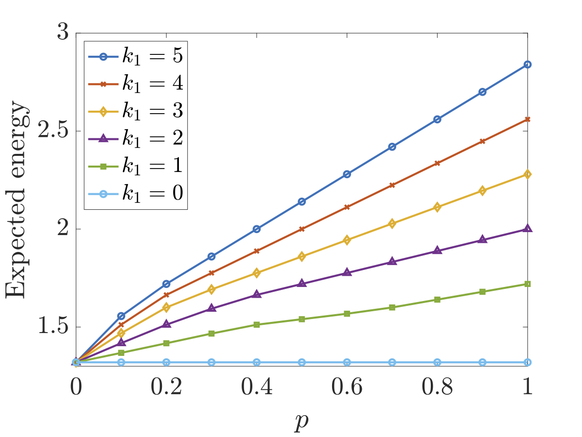
In the figures below we have plotted both the optimal expected time and energy the scheduler can ensure when there are different number of faults in each processor as the parameter p (the probability of a fault causing a failure) varies. As would be expected, both the optimal expected time and energy consumption increases both as the number of faults increases and the probability that a fault causes a failure increases.
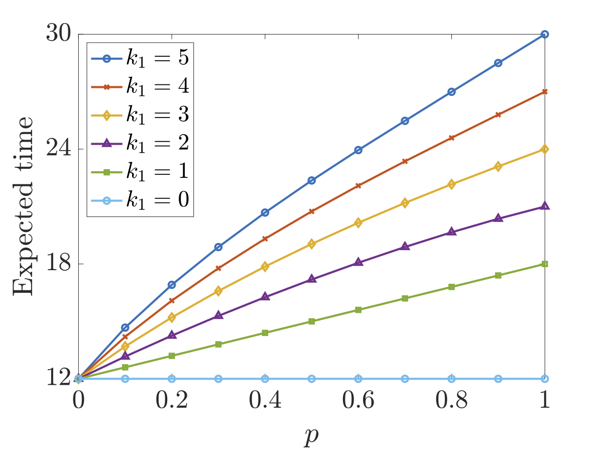
Considering the synthesised optimal schedulers for the expected time case, when k1=k2=1 and p=1, the optimal approach is to just use the faster processor P1 and the expected time equals 18.0. The optimal strategy for the environment, i.e., the choices that yield the worst-case expected time, against this scheduler is to delay all tasks as long as possible and cause a fault when a multiplication task is just about to complete on P1 (recall P2 is never used under the optimal scheduler). A multiplication is chosen as this takes longer (3 picoseconds) than an addition task (2 picoseconds). These choices can be seen through the fact that 18.0 is the time for 4 multiplications and 3 additions to be performed on P1, while the problem requires 3 multiplications and 3 additions. As soon as the probability of a fault causing a failure is less than 1, the optimal scheduler does use processor P2 from the beginning by initially scheduling task1 on process P1 and task2 on processor P2 (which is also optimal when no faults can occur).
In the case of the expected energy consumption, the optimal scheduler uses both processes unless one has 2 or more faults than the other and there is only a small chance that a fault will cause a failure. For example, if P1 has 3 faults and P2 has 1 fault, then P1 is only used by the optimal scheduler when the probability of a failure causing a fault is approximately 0.25 or less.