
Related publications: [KNP12a]
In this case study we consider a number of self-stabilising algorithms from the literature.
A self-stabilising protocol for a network of processes is a protocol which, when started from some possibly illegal start configuration, returns to a legal/stable configuration without any outside intervention within some finite number of steps. For further details on self-stabilisation see here.
In each of the protocols we consider, the network is a ring of identical processes. The stable configurations are those where there is exactly one process designated as "privileged" (has a token). This privilege (token) should be passed around the ring forever in a fair manner.
For each of the protocols, we compute the minimum probability of reaching a stable configuration and the maximum expected time (number of steps) to reach a stable configuration (given that the above probability is 1) over every possible initial configuration of the protocol.
The first protocol we consider is due to Herman [Her90]. The protocol operates synchronously, the ring is oriented, and communication is unidirectional in the ring. In this protocol the number of processes in the ring must be odd.
Each process in the ring has a local boolean variable xi, and there is a token in place i if xi=x(i-1). In a basic step of the protocol, if the current values of xi and x(i-1) are equal, then it makes a (uniform) random choice as to the next value of xi, and otherwise it sets it equal to the current value of x(i-1).
By way of example, the PRISM source code for the case where there are three processes in the ring is given below.
// herman's self stabilising algorithm [Her90]
// gxn/dxp 13/07/02

// the procotol is synchronous with no nondeterminism (a DTMC)
dtmc

const double p = 0.5;

// module for process 1
module process1

	// Boolean variable for process 1
	x1 : [0..1];

	[step]  (x1=x3) -> p : (x1'=0) + 1-p : (x1'=1);
	[step] !(x1=x3) -> (x1'=x3);

endmodule

// add further processes through renaming
module process2 = process1 [ x1=x2, x3=x1 ] endmodule
module process3 = process1 [ x1=x3, x3=x2 ] endmodule

// cost - 1 in each state (expected number of steps)
rewards "steps"
	true : 1;
endrewards

// set of initial states: all (i.e. any possible initial configuration of tokens)
init
	true
endinit

// formula, for use in properties: number of tokens
// (i.e. number of processes that have the same value as the process to their left)
formula num_tokens = (x1=x2?1:0)+(x2=x3?1:0)+(x3=x1?1:0);

// label - stable configurations (1 token)
label "stable" = num_tokens=1;
The table below shows statistics for protocol we have built for different numbers of processes (size of the ring). The first section gives the number of states and transitions in the DTMC representing the model. The second part refers to the MTBDD used to store it: the total number of nodes and the number of leaves (terminal nodes).
| N: | Model: | MTBDD: | ||||
| States: | Transitions: | Nodes: | Leaves: | |||
| 3 | 8 | 28 | 24 | 3 | ||
| 5 | 32 | 244 | 75 | 4 | ||
| 7 | 128 | 2,188 | 158 | 5 | ||
| 9 | 512 | 19,684 | 273 | 6 | ||
| 11 | 2,048 | 177,148 | 420 | 7 | ||
| 13 | 8,192 | 1,594,324 | 599 | 8 | ||
| 15 | 32,768 | 14,348,908 | 810 | 9 | ||
| 17 | 131,072 | 129,140,164 | 1,053 | 10 | ||
| 19 | 524,288 | 1,162,261,468 | 1,328 | 11 | ||
| 21 | 2,097,152 | 10,460,353,204 | 1,635 | 12 | ||
We first check the correctness of the protocol, namely that:
We then study its performance, in particular:
For the latter, we consider the worst-case behaviour over all possible initial configurations and over all initial configurations with k tokens.
These properties can be expressed in PRISM as follows.
const int k; // number of tokens
const int K; // number of steps

// labels
label "k_tokens" = num_tokens=k; // configurations with k tokens

// From any configuration, a stable configuration is reached with probability 1
filter(forall, "init" => P>=1 [ F "stable" ])

// Maximum expected time to reach a stable configuration (for all configurations)
R=? [ F "stable" {"init"}{max} ]

// Maximum/minimum expected time to reach a stable configuration (for all k-token configurations)
R=? [ F "stable" {"k_tokens"}{max} ]
R=? [ F "stable" {"k_tokens"}{min} ]
The minimum probability of reaching a stable state is 1 for all models built (up to N = 21).
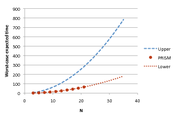
The worst-case expected time, over all initial configurations, is shown in the plot below (marked "PRISM"). For comparison, we also plot the upper bound on this value proved by Kiefer et al. [KMO+11] of (approximately) 0.64N2. As the graph illustrates, the actual worst-case value is considerably lower. Elsewhere, McIver and Morgan [MM05a] showed that the the worst-case time for initial configurations with 3 tokens is 4abc/N, where a, b and c are the distances between the three tokens. This therefore represents a lower bound on the worst-case expected time and is also shown in the plot. Kiefer, conjecture that this represents the worst-case for any number of tokens. Our results corroborate this conjecture precisely for all models built.
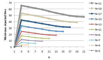
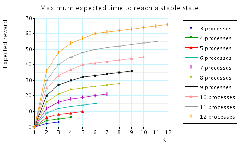
Further evidence of the correctness of McIver and Morgan's conjecture is shown in the graph below, where we plot, as k varies, the maximum expected time to reach a stable configuration given that the initial number of tokens equals k. As can be seen, for all models up to N = 21, the worst case is for k = 3 tokens and the maximum expected time decreases for increasing values of k.
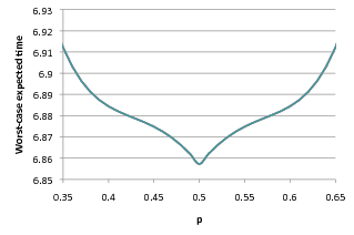
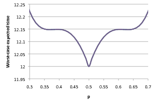
Lastly, we examine the effect of the probabilistic value used for the random choice in Herman's algorithm (p in the PRISM code above).
As the plot below indicates, for values of N = 9 or below, p = 0.5 is the optimum value. However, interestingly, for larger values of N, this does not hold. In fact, in these case, values of p other than 0.5 (i.e. biased coins) result in better performance (lower expected execution time) for the protocol.
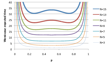
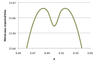
Moreover, zooming in on the above plots reveals unexpected trends for values of p close to 0.5:
|
|
| |
See [KNP12a] for further results on this model.
The protocol we consider in this section is due to Israeli and Jalfon [IJ90]. It operates asynchronously with an arbitrary scheduler, the ring is oriented and communication is bidirectional in the ring.
Each process has a boolean variable qi which represents the fact that a token is in place i. A process is active if it has a token and only active processes can be scheduled. When an active process is scheduled, it makes a (uniform) random choice as to whether to move the token to its left or right. Note that if a process ends up with two tokens, these tokens are merged into a single token.
By way of example, the PRISM source code for the case where there are three processes in the ring is given below.
// Israeli-Jalfon self stabilising algorithm
// dxp/gxn 10/06/02

mdp

// variables to represent whether a process has a token or not
// note they are global because they can be updated by other processes
global q1  : [0..1];
global q2  : [0..1];
global q3  : [0..1];

// module of process 1
module process1

	[] (q1=1) -> 0.5 : (q1'=0) & (q3'=1) + 0.5 : (q1'=0) & (q2'=1);

endmodule

// add further processes through renaming
module process2 = process1 [ q1=q2, q2=q3, q3=q1 ] endmodule
module process3 = process1 [ q1=q3, q2=q1, q3=q2 ] endmodule

// cost - 1 in each state (expected steps)
rewards "steps"
	true : 1;
endrewards

// formula, for use here and in properties: number of tokens
formula num_tokens = q1+q2+q3;

// initial states (at least one token)
init
	num_tokens >= 1
endinit
The table below shows statistics for protocol we have built for different numbers of processes (size of the ring). The first section gives the number of states in the MDP representing the model. The second part refers to the MTBDD which represents this MDP: the total number of nodes and the number of leaves (terminal nodes).
| N: | Model: | MTBDD: | |||
| States: | Nodes: | Leaves: | |||
| 3 | 7 | 48 | 3 | ||
| 4 | 15 | 85 | 3 | ||
| 5 | 31 | 129 | 3 | ||
| 6 | 63 | 177 | 3 | ||
| 7 | 127 | 229 | 3 | ||
| 8 | 255 | 285 | 3 | ||
| 9 | 511 | 345 | 3 | ||
| 10 | 1,023 | 409 | 3 | ||
| 11 | 2,047 | 477 | 3 | ||
| 12 | 4,095 | 549 | 3 | ||
| 13 | 8,191 | 625 | 3 | ||
| 14 | 16,383 | 705 | 3 | ||
| 15 | 32,767 | 789 | 3 | ||
| 16 | 65,535 | 877 | 3 | ||
| 17 | 131,071 | 969 | 3 | ||
| 18 | 262,143 | 1,065 | 3 | ||
| 19 | 524,287 | 1,165 | 3 | ||
| 20 | 1,048,575 | 1,269 | 3 | ||
| 21 | 2,097,151 | 1,377 | 3 | ||
We analysed the protocol through the following properties.
Which can be expressed in PRISM as follows.
const int k; // number of tokens
const int K; // number of steps

// labels
label "k_tokens" = num_tokens=k; // configurations with k tokens

// From any configuration, a stable configuration is reached with probability 1
filter(forall, "init" => P>=1 [ F "stable" ])

// Maximum expected time to reach a stable configuration (for all configurations)
Rmax=? [ F "stable" {"init"}{max} ]

// Maximum/minimum expected time to reach a stable configuration (for all k-token configurations)
Rmax=? [ F "stable" {"k_tokens"}{max} ]
Rmin=? [ F "stable" {"k_tokens"}{min} ]

// Minimum probability reached a stable configuration within K steps (for all configurations)
Pmin=? [ F<=K "stable" {"init"}{min} ]
The table below gives the model checking statistics when checking that from any configuration, a stable configuration is reached with probability 1 and calculating the maximum expected time to reach a stable configuration.
| N: | A stable configuration is reached with probability 1 | Maximum expected time to reach a stable configuration | ||||
| Iterations: | Result: | Iterations: | Result: | |||
| 3 | 3 | true | 21 | 3.0 | ||
| 4 | 5 | true | 39 | 6.0 | ||
| 5 | 7 | true | 61 | 10.0 | ||
| 6 | 9 | true | 87 | 15.0 | ||
| 7 | 12 | true | 116 | 21.0 | ||
| 8 | 14 | true | 149 | 28.0 | ||
| 9 | 16 | true | 186 | 36.0 | ||
| 10 | 19 | true | 226 | 45.0 | ||
| 11 | 23 | true | 270 | 55.0 | ||
| 12 | 25 | true | 317 | 66.0 | ||
| 13 | 28 | true | 367 | 78.0 | ||
| 14 | 31 | true | 420 | 91.0 | ||
| 15 | 35 | true | 477 | 105.0 | ||
| 16 | 38 | true | 537 | 120.0 | ||
| 17 | 41 | true | 599 | 136.0 | ||
| 18 | 44 | true | 665 | 153.0 | ||
| 19 | 48 | true | 733 | 171.0 | ||
| 20 | 52 | true | 805 | 190.0 | ||
| 21 | 55 | true | 879 | 210.0 | ||
In all the cases considered, the configurations which achieve the maximum expected time are those where all the processes have tokens. To illustrate this fact, in the graph below we have plotted, as k varies, the maximum expected time to reach a stable configuration given that the initial number of tokens equals k.
In addition, below we have plotted the minimum expected time to reach a stable configuration given that the initial number of tokens k.
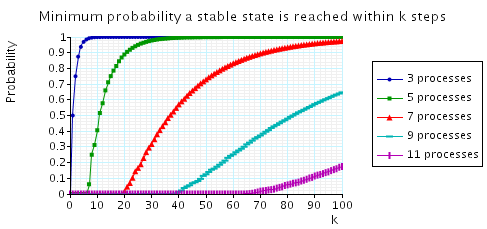
Lastly, we have also plotted the minimum probability of reaching a stable configuration within k steps.
Now we consider the self-stabilising protocol of Beauquier, Gradinariu and Johnen [BGJ99] for an arbitrary scheduler. It operates asynchronously, the ring is oriented, communication is unidirectional in the ring, and the number processes in the ring must be odd.
Each process two boolean variables: di and pi where:
The stable configurations are those where there is only one probabilistic token. A process is active if it has a deterministic token and only active processes can be scheduled. When an active process is scheduled, it sets di to be the negation of it current value (passes the deterministic token), and if it also has a probabilistic token, it makes a (uniform) random choice as to the next value of pi (randomly selects whether to pass the probabilistic token or not).
By way of example, the PRISM source code for the case where there are three processes in the ring is given below.
// self stabilisation algorithm Beauquier, Gradinariu and Johnen
// gxn/dxp 18/07/02

mdp

// module of process 1
module process1

	d1 : bool; // probabilistic variable
	p1 : bool; // deterministic variable

	[] d1=d3 &  p1=p3 -> 0.5 : (d1'=!d1) & (p1'=p1) + 0.5 : (d1'=!d1) & (p1'=!p1);
	[] d1=d3 & !p1=p3 -> (d1'=!d1);

endmodule

// add further processes through renaming
module process2 = process1 [ p1=p2, p3=p1, d1=d2, d3=d1 ] endmodule
module process3 = process1 [ p1=p3, p3=p2, d1=d3, d3=d2 ] endmodule

// cost - 1 in each state (expected steps)
rewards "steps"
	true : 1;
endrewards

// initial states - any state with more than 1 token, that is all states
init
	true
endinit

// formula, for use in properties: number of tokens
formula num_tokens = (p1=p2?1:0)+(p2=p3?1:0)+(p3=p1?1:0);
The table below shows statistics for protocol we have built for different numbers of processes (size of the ring). The first section gives the number of states in the MDP representing the model. The second part refers to the MTBDD which represents this MDP: the total number of nodes and the number of leaves (terminal nodes).
| N: | Model: | MTBDD: | |||
| States: | Nodes: | Leaves: | |||
| 3 | 64 | 141 | 3 | ||
| 5 | 1,024 | 336 | 3 | ||
| 7 | 16,384 | 559 | 3 | ||
| 9 | 262,144 | 810 | 3 | ||
| 11 | 4,194,304 | 1,089 | 3 | ||
The table below gives the model checking statistics when calculating, over all configurations, the minimum probability that a stable configuration is reached and the maximum expected time to reach a stable configuration.
| N: | A stable configuration is reached with probability 1 | Maximum expected time to reach a stable configuration | ||||
| Iterations: | Result: | Iterations: | Result: | |||
| 3 | 2 | true | 20 | 2.00 | ||
| 5 | 8 | true | 64 | 11.9 | ||
| 7 | 21 | true | 170 | 37.8 | ||
| 9 | 40 | true | 380 | 84.4 | ||
| 11 | 65 | true | 732 | 162 | ||
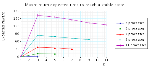
In all the cases considered, the configurations which achieve the maximum expected time are those where only three processes have probabilistic tokens. To illustrate this fact, in the graph below we have plotted, as k varies, the maximum expected time to reach a stable configuration given that the initial number of tokens k.
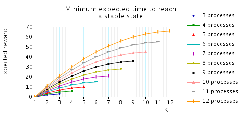
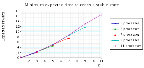
In addition, below we have plotted the minimum expected time to reach a stable configuration given that the initial number of tokens equals k.
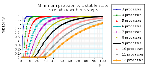
Lastly, we have also plotted the minimum probability of reaching a stable configuration within k steps.