
(Ciardo & Trivedi)
This case study is based on the flexible manufacturing system of [CT93]. The model is represented as a CTMC. We use N to denote the number of tokens in the system. The PRISM source code for this case study given below.
// flexible manufacturing system [CT93]
// gxn/dxp 11/06/01

ctmc

const int n; // number of tokens

// rates from Pi equal #(Pi) * min(1, np/r)
// where np = (3n)/2 and r = P1+P2+P3+P12
const int np=floor((3*n)/2);
formula r = P1+P2+P3+P12;

module machine1

	P1 : [0..n] init n;
	P1wM1 : [0..n];
	P1M1 : [0..3];
	P1d : [0..n];
	P1s : [0..n];
	P1wP2 : [0..n];
	M1 : [0..3] init 3;

	[t1] (P1>0) & (M1>0) & (P1M1<3)  -> P1*min(1,np/r) : (P1'=P1-1) & (P1M1'=P1M1+1) & (M1'=M1-1);
	[t1] (P1>0) & (M1=0) & (P1wM1<n) -> P1*min(1,np/r) : (P1'=P1-1) & (P1wM1'=P1wM1+1);

	[] (P1M1>0) & (P1wM1=0) & (M1<3) & (P1s<n) -> 0.2*P1M1 : (P1M1'=P1M1-1) & (M1'=M1+1) & (P1s'=P1s+1);
	[] (P1M1>0) & (P1wM1>0) & (P1s<n) -> 0.2*P1M1 : (P1wM1'=P1wM1-1) & (P1s'=P1s+1);

	[] (P1M1>0) & (P2wP1=0) & (P1wM1=0) & (M1<3) & (P1wP2<n) -> 0.05*P1M1 : (P1M1'=P1M1-1) & (M1'=M1+1) & (P1wP2'=P1wP2+1);
	[] (P1M1>0) & (P2wP1=0) & (P1wM1>0) & (P1wP2<n) -> 0.05*P1M1 : (P1wM1'=P1wM1-1) & (P1wP2'=P1wP2+1);

	[p1p2] (P1M1>0) & (P2wP1>0) & (P1wM1=0) & (M1<3) -> 0.05*P1M1 : (P1M1'=P1M1-1) & (M1'=M1+1);
	[p1p2] (P1M1>0) & (P2wP1>0) & (P1wM1>0) -> 0.05*P1M1 : (P1wM1'=P1wM1-1);

	[p1p2] (P1wP2>0)  -> 1: (P1wP2'=P1wP2-1);
	[]     (P1s>0) & (P1+P1s<=n) -> 1/60 : (P1s'=0) & (P1'=P1+P1s);
	[fp12] (P1+P12s<=n) -> 1: (P1'=P1+P12s);

endmodule

module machine2

	P2 : [0..n] init n;
	P2wM2 : [0..n];
	P2M2 : [0..1];
	P2s : [0..n];
	P2wP1 : [0..n];
	M2 : [0..1] init 1;

	[t2] (P2>0) & (M2>0) & (P2M2<1)  -> P2*min(1,np/r) : (P2'=P2-1) & (P2M2'=P2M2+1) & (M2'=M2-1);
	[t2] (P2>0) & (M2=0) & (P2wM2<n) -> P2*min(1,np/r) : (P2'=P2-1) & (P2wM2'=P2wM2+1);

	[] (P2M2>0) & (P2wM2=0) & (M2<1) & (P2s<n) -> 0.1 : (P2M2'=P2M2-1) & (M2'=M2+1) & (P2s'=P2s+1);
	[] (P2M2>0) & (P2wM2>0) & (P2s<n) -> 0.1 : (P2wM2'=P2wM2-1) & (P2s'=P2s+1);

	[] (P2M2>0) & (P1wP2=0) & (P2wM2=0) & (M2<1) & (P2wP1<n) -> 1/15: (P2M2'=P2M2-1) & (M2'=M2+1) & (P2wP1'=P2wP1+1);
	[] (P2M2>0) & (P1wP2=0) & (P2wM2>0) & (P2wP1<n) -> 1/15: (P2wM2'=P2wM2-1) & (P2wP1'=P2wP1+1);

	[p1p2] (P2M2>0) & (P1wP2>0) & (P2wM2=0) & (M2<1) -> 1/15: (P2M2'=P2M2-1) & (M2'=M2+1);
	[p1p2] (P2M2>0) & (P1wP2>0) & (P2wM2>0) -> 1/15: (P2wM2'=P2wM2-1);

	[p1p2] (P2wP1>0) -> 1 : (P2wP1'=P2wP1-1);
	[]     (P2s>0) & (P2+P2s<=n) -> 1/60 : (P2s'=0) & (P2'=P2+P2s);
	[fp12] (P2+P12s<=n) -> 1 : (P2'=P2+P12s);
	[p2p3] (M2>0) -> 1 : (M2'=M2);

endmodule

module machine3

	P3 : [0..n] init n;
	P3M2 : [0..n];
	P3s : [0..n];

	[t3] (P3>0) & (P3M2<n) -> P3*min(1,np/r) : (P3'=P3-1) & (P3M2'=P3M2+1);

	[p2p3] (P3M2>0) & (P3s<n) -> 1/2 : (P3M2'=P3M2-1) & (P3s'=P3s+1);
	[]     (P3s>0) & (P3+P3s<=n) -> 1/60 : (P3s'=0) & (P3'=P3+P3s);

endmodule

module machine12

	P12 : [0..n];
	P12wM3 : [0..n];
	P12M3 : [0..2];
	P12s : [0..n];
	M3 : [0..2] init 2;

	[p1p2] (P12<n) -> 1: (P12'=P12+1);

	[t12] (P12>0) & (M3>0) & (P12M3<2) -> P12*min(1,np/r) : (P12'=P12-1) & (P12M3'=P12M3+1) & (M3'=M3-1);
	[t12] (P12>0) & (M3=0) & (P12wM3<n) -> P12*min(1,np/r) : (P12'=P12-1) & (P12wM3'=P12wM3+1);

	[] (P12M3>0) & (P12wM3=0) & (P12s<n) & (M3<2) -> P12M3 : (P12M3'=P12M3-1) & (P12s'=P12s+1) & (M3'=M3+1);
	[] (P12M3>0) & (P12wM3>0) & (P12s<n) -> P12M3 : (P12wM3'=P12wM3-1) & (P12s'=P12s+1);

	[fp12] (P12s>0) -> 1/60 : (P12s'=0);

endmodule

// reward structures

// throughput of machine1
rewards "throughput_m1"
	[t1]  true : 1;
endrewards
// throughput of machine2
rewards "throughput_m2"
	[t2]  true : 1;
endrewards
// throughput of machine3
rewards "throughput_m3"
	[t3]  true : 1;
endrewards
// throughput of machine12
rewards "throughput_m12"
	[t12]  true : 1;
endrewards
// productivity of the system
rewards "productivity"
	[t1]  true : 400;
	[t2]  true : 600;
	[t3]  true : 100;
	[t12] true : 1100;
endrewards
The table below shows statistics for each model we have built. The first section gives information about the CTMC representing the model: the number of states and the number of non zeros (transitions). The second part refers to the MTBDD which represents this CTMC: the total number of nodes, the number of leaves (terminal nodes), and the amount of memory needed to store it. The last column gives the amount of memory a sparse matrix would need to represent the same CTMC.
| N: | Model: | MTBDD: | Sparse: | ||||||
| States: | NNZ: | Nodes: | Leaves: | Kb: | Kb: | ||||
| 1 | 54 | 155 | 783 | 9 | 15.3 | 2.03 | |||
| 2 | 810 | 3,699 | 4,371 | 14 | 85.4 | 46.5 | |||
| 3 | 6,520 | 37,394 | 10,896 | 22 | 212 | 463 | |||
| 4 | 35,910 | 237,120 | 28,470 | 30 | 556 | 2,919 | |||
| 5 | 152,712 | 1,111,482 | 50,877 | 43 | 992 | 13,621 | |||
| 6 | 537,768 | 4,205,670 | 78,125 | 53 | 1,526 | 51,385 | |||
| 7 | 1,639,440 | 13,552,968 | 120,834 | 71 | 2,360 | 165,227 | |||
| 8 | 4,459,455 | 38,533,968 | 215,250 | 84 | 4,204 | 468,989 | |||
| 9 | 11,058,190 | 99,075,405 | 309,067 | 108 | 6,032 | 1,204,235 | |||
| 10 | 25,397,658 | 234,523,289 | 406,018 | 126 | 7,930 | 2,847,529 | |||
The table below gives the times taken to construct the models. This process involves first building a CTMC (represented as an MTBDD) from the system description (in our module based language), and then computing the reachable states using a BDD based fixpoint algorithm. The total time required and the number of fixpoint iterations are given below.
| N: | Construction: | ||
| Time (s): | Iter.s: | ||
| 1 | 0.173 | 9 | |
| 2 | 0.449 | 17 | |
| 3 | 0.829 | 25 | |
| 4 | 2.62 | 33 | |
| 5 | 5.25 | 41 | |
| 6 | 14.2 | 49 | |
| 7 | 35.8 | 57 | |
| 8 | 44.2 | 65 | |
| 9 | 61.0 | 73 | |
| 10 | 93.7 | 81 | |
We now report on the model checking results obtained using PRISM when verifying the following CSL properties.
// expected throughput of each machine
R{"throughput_m1"}=?  [ S ]
R{"throughput_m2"}=?  [ S ]
R{"throughput_m3"}=?  [ S ]
R{"throughput_m12"}=? [ S ]

// expected productivity of the system
R{"productivity"}=? [ S ]
All experiments were carried out on a 2.80GHz PC with 1 Gb memory running Linux and in all iterative methods we stop iterating when the relative error between subsequent iteration vectors is less than 1e-6, that is:
The table below gives the times taken to compute the steady state probabilities using both the Jacobi and (backwards) Gauss Seidel methods.
The number of iterations required and the time taken using the MTBDD, sparse and hybrid engines is as follows.
| N: | Jacobi: | Gauss Seidel: | ||||||||
| Iterations: | Time per iteration: (s) | Iterations: | Time per iteration: (s) | |||||||
| MTBDD | Sparse | Hybrid | Sparse | Hybrid | ||||||
| 1 | 434 | 0.004788 | < 0.00001 | 0.000005 | 75 | < 0.00001 | < 0.00001 | |||
| 2 | 378 | 0.154611 | 0.000032 | 0.000040 | 92 | 0.000043 | 0.000087 | |||
| 3 | 554 | 1.626347 | 0.000343 | 0.000388 | 106 | 0.000557 | 0.000943 | |||
| 4 | 729 | - | 0.001771 | 0.003660 | 118 | 0.002610 | 0.005992 | |||
| 5 | 905 | - | 0.008700 | 0.023281 | 127 | 0.011992 | 0.027898 | |||
| 6 | 1,080 | - | 0.033600 | 0.084465 | 136 | 0.044419 | 0.104735 | |||
| 7 | 1,258 | - | 0.109400 | 0.260022 | 144 | 0.143736 | 0.331993 | |||
| 8 | 1,438 | - | 0.325950 | 0.887426 | 151 | 0.420152 | 0.949457 | |||
| 9 | 1,619 | - | 0.865450 | 3.712932 | 159 | 1.077013 | 2.335075 | |||
| 10 | 1,804 | - | - | 10.00491 | 166 | - | 5.505777 | |||
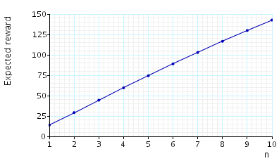
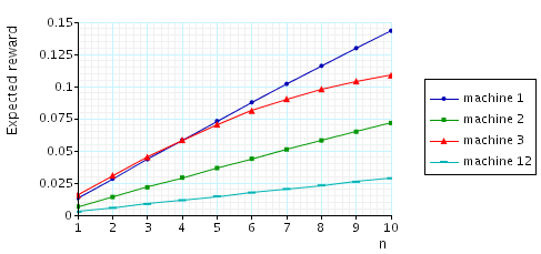
The graphs below present the results obtained for the different CSL properties.
The expected throughput of each machine:
The expected productivity of the system: