Related publications: [KNS03b]
This case study concerns the Tree Identify Protocol of the IEEE 1394 High Performance Serial Bus (called ``FireWire''). The 1394 High Performance serial bus is used to transport video and audio signals within a network of multimedia devices. It has a scalable architecture and is ``hot-pluggable'', meaning that at any time devices can easily be added or removed from the network.
The tree identify process of IEEE 1394 is a leader election protocol which takes place after a bus reset in the network, that is, when a node is added or removed from the network. After such a reset all nodes in the network have equal status, and know only to which nodes they are directly connected. A leader (root) needs to be chosen to act as the manager of the bus for subsequent phases of IEEE 1394. This is done by the nodes communicating ``be my parent'' messages, starting from the leaf nodes. It can happen that two nodes contend the leadership (root contention), in which case the contenders exchange additional messages and involve time delays and electronic coin tosses.
The protocol is designed for use on connected networks, will correctly elect a leader if the network is acyclic, and will report an error if a cycle is detected.
In our analysis, we will consider two cases for the maximum transmission delay along the wires (the constant delay): 360 nanoseconds (ns) and 30ns. This models the distance between the two nodes, i.e. the length of the connecting wires. A delay of 360ns represents the assumption that the nodes are separated by a distance close to the maximum required for the correctness of the protocol. A delay of 30ns corresponds more closely to the maximum separation of nodes specified in the actual IEEE standard. In fact, in the second case, the correct value is 22.725ns so our figure of 30ns is an over-approximation. This is for efficiency reasons: it allows us to use a time granularity of 10ns when we consider probabilistic model checking using digital clocks. In the following paragraphs, we will refer to the two cases (360ns and 30ns) as `long wire' and `short wire', respectively.
For further information concerning the IEEE 1394 Tree Identify Protocol see here.
We consider the following probabilistic timed automata models of the root contention part of the tree identify protocol, which are based on probabilistic I/O automata models presented in [SV99].
For details on the correctness of the integer semantics when verifying probabilistic timed automata against performance measures see [KNS02a, KNPS06], and, in the case of the region graph semantics, see [KNSS02].
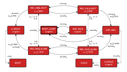
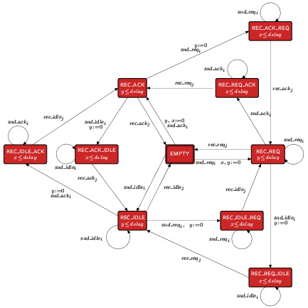
Impl: which consists of the parallel composition of two nodes (Node1 and Node2), and two communication channels (Wire12 for messages from Node1 to Node2, and Wire21 for messages from Node2 to Node1) and corresponds to the system Impl of [SV99].
The probabilistic timed automaton representing Nodei is given below.
The probabilistic timed automaton for the communication channel Wireij is given below.
We have constructed an MDP for this model using the integer semantics approach [KNS03b, KNPS06]. The PRISM source code is given below.
// firewire protocol with integer semantics
// dxp/gxn 14/06/01

mdp

// CLOCKS
// x1 (x2) clock for node1 (node2)
// y1 and y2 (z1 and z2) clocks for wire12 (wire21)

// maximum and minimum delays
// fast
const int rc_fast_max = 85;
const int rc_fast_min = 76;
// slow
const int rc_slow_max = 167;
const int rc_slow_min = 159;
// delay caused by the wire length
const int delay;
// probability of choosing fast
const double fast;
const double slow=1-fast;

module wire12

	// local state
	w12 : [0..9];
	// 0 - empty
	// 1 -	rec_req
	// 2 -  rec_req_ack
	// 3 -	rec_ack
	// 4 -	rec_ack_idle
	// 5 -	rec_idle
	// 6 -	rec_idle_req
	// 7 -	rec_ack_req
	// 8 -	rec_req_idle
	// 9 -	rec_idle_ack

	// clock for wire12
	y1 : [0..delay+1];
	y2 : [0..delay+1];

	// empty
	// do not need y1 and y2 to increase as always reset when this state is left
	// similarly can reset y1 and y2 when we re-enter this state
	[snd_req12]  w12=0 -> (w12'=1) & (y1'=0) & (y2'=0);
	[snd_ack12]  w12=0 -> (w12'=3) & (y1'=0) & (y2'=0);
	[snd_idle12] w12=0 -> (w12'=5) & (y1'=0) & (y2'=0);
	[time]       w12=0 -> (w12'=w12);
	// rec_req
	[snd_req12]  w12=1 -> (w12'=1);
	[rec_req12]  w12=1 -> (w12'=0) & (y1'=0) & (y2'=0);
	[snd_ack12]  w12=1 -> (w12'=2) & (y2'=0);
	[snd_idle12] w12=1 -> (w12'=8) & (y2'=0);
	[time]       w12=1 & y2<delay ->  (y1'=min(y1+1,delay+1)) & (y2'=min(y2+1,delay+1));
	// rec_req_ack
	[snd_ack12] w12=2 -> (w12'=2);
	[rec_req12] w12=2 -> (w12'=3);
	[time]      w12=2 & y1<delay ->  (y1'=min(y1+1,delay+1)) & (y2'=min(y2+1,delay+1));
	// rec_ack
	[snd_ack12]  w12=3 -> (w12'=3);
	[rec_ack12]  w12=3 -> (w12'=0) & (y1'=0) & (y2'=0);
	[snd_idle12] w12=3 -> (w12'=4) & (y2'=0);
	[snd_req12]  w12=3 -> (w12'=7) & (y2'=0);
	[time]       w12=3 & y2<delay ->  (y1'=min(y1+1,delay+1)) & (y2'=min(y2+1,delay+1));
	// rec_ack_idle
	[snd_idle12] w12=4 -> (w12'=4);
	[rec_ack12]  w12=4 -> (w12'=5);
	[time]       w12=4 & y1<delay ->  (y1'=min(y1+1,delay+1)) & (y2'=min(y2+1,delay+1));
	// rec_idle
	[snd_idle12] w12=5 -> (w12'=5);
	[rec_idle12] w12=5 -> (w12'=0) & (y1'=0) & (y2'=0);
	[snd_req12]  w12=5 -> (w12'=6) & (y2'=0);
	[snd_ack12]  w12=5 -> (w12'=9) & (y2'=0);
	[time]       w12=5 & y2<delay ->  (y1'=min(y1+1,delay+1)) & (y2'=min(y2+1,delay+1));
	// rec_idle_req
	[snd_req12]  w12=6 -> (w12'=6);
	[rec_idle12] w12=6 -> (w12'=1);
	[time]       w12=6 & y1<delay ->  (y1'=min(y1+1,delay+1)) & (y2'=min(y2+1,delay+1));
	// rec_ack_req
	[snd_req12] w12=7 -> (w12'=7);
	[rec_ack12] w12=7 -> (w12'=1);
	[time]      w12=7 & y1<delay ->  (y1'=min(y1+1,delay+1)) & (y2'=min(y2+1,delay+1));
	// rec_req_idle
	[snd_idle12] w12=8 -> (w12'=8);
	[rec_req12]  w12=8 -> (w12'=5);
	[time]       w12=8 & y1<delay ->  (y1'=min(y1+1,delay+1)) & (y2'=min(y2+1,delay+1));
	// rec_idle_ack
	[snd_ack12]  w12=9 -> (w12'=9);
	[rec_idle12] w12=9 -> (w12'=3);
	[time]       w12=9 & y1<delay ->  (y1'=min(y1+1,delay+1)) & (y2'=min(y2+1,delay+1));

endmodule

module node1

	// clock for node1
	x1 : [0..168];

	// local state
	s1 : [0..8];
	// 0 - root contention
	// 1 - rec_idle
	// 2 - rec_req_fast
	// 3 - rec_req_slow
	// 4 - rec_idle_fast
	// 5 - rec_idle_slow
	// 6 - snd_req
	// 7- almost_root
	// 8 - almost_child

	// added resets to x1 when not considered again until after rest
	// removed root and child (using almost root and almost child)

	// root contention immediate state)
	[snd_idle12] s1=0 -> fast : (s1'=2) & (x1'=0) +  slow : (s1'=3) & (x1'=0);
	[rec_idle21] s1=0 -> (s1'=1);
	// rec_idle immediate state)
	[snd_idle12] s1=1 -> fast : (s1'=4) & (x1'=0) +  slow : (s1'=5) & (x1'=0);
	[rec_req21]  s1=1 -> (s1'=0);
	// rec_req_fast
	[rec_idle21] s1=2 -> (s1'=4);
	[snd_ack12]  s1=2 & x1>=rc_fast_min -> (s1'=7) & (x1'=0);
	[time]       s1=2 & x1<rc_fast_max -> (x1'=min(x1+1,168));
	// rec_req_slow
	[rec_idle21] s1=3 -> (s1'=5);
	[snd_ack12]  s1=3 & x1>=rc_slow_min -> (s1'=7) & (x1'=0);
	[time]       s1=3 & x1<rc_slow_max -> (x1'=min(x1+1,168));
	// rec_idle_fast
	[rec_req21] s1=4 -> (s1'=2);
	[snd_req12] s1=4 & x1>=rc_fast_min -> (s1'=6) & (x1'=0);
	[time]      s1=4 & x1<rc_fast_max -> (x1'=min(x1+1,168));
	// rec_idle_slow
	[rec_req21] s1=5 -> (s1'=3);
	[snd_req12] s1=5 & x1>=rc_slow_min -> (s1'=6) & (x1'=0);
	[time]      s1=5 & x1<rc_slow_max -> (x1'=min(x1+1,168));
	// snd_req
	// do not use x1 until reset (in state 0 or in state 1) so do not need to increase x1
	// also can set x1 to 0 upon entering this state
	[rec_req21] s1=6 -> (s1'=0);
	[rec_ack21] s1=6 -> (s1'=8);
	[time]      s1=6 -> (s1'=s1);
	// almost root (immediate)
	// loop in final states to remove deadlock
	[] s1=7 & s2=8 -> (s1'=s1);
	[] s1=8 & s2=7 -> (s1'=s1);
	[time] s1=7 -> (s1'=s1);
	[time] s1=8 -> (s1'=s1);

endmodule

// construct remaining automata through renaming
module wire21=wire12[w12=w21, y1=z1, y2=z2,
	snd_req12=snd_req21, snd_idle12=snd_idle21, snd_ack12=snd_ack21,
	rec_req12=rec_req21, rec_idle12=rec_idle21, rec_ack12=rec_ack21]
endmodule
module node2=node1[s1=s2, s2=s1, x1=x2,
	rec_req21=rec_req12, rec_idle21=rec_idle12, rec_ack21=rec_ack12,
	snd_req12=snd_req21, snd_idle12=snd_idle21, snd_ack12=snd_ack21]
endmodule

// reward structure for expected time
rewards "time"
	[time] true : 1;
endrewards
Abst: which is represented by a single probabilistic timed automaton given below where each instance of bifurcating edges corresponds to a coin being flipped. This model is an abstraction of Impl based on the the probabilistic I/O automaton I1 of [SV99].
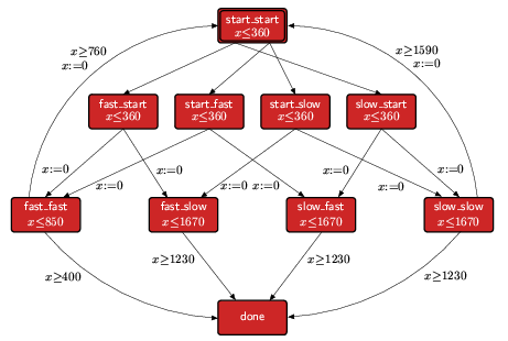
We have constructed MDP models for this system using integer semantics [KNS03b, KNPS06] and the region graph semantics of [KNSS02]. The PRISM source code for the integer semantics model is given below.
// discrete version of abstract firewire protocol
// gxn 23/05/2001

mdp

// wire delay
const int delay;

// probability of choosing fast and slow
const double fast;
const double slow = 1-fast;

// maximal constant
const int kx = 167;

module abstract_firewire

	// clock
	x : [0..kx+1];

	// local state
	s : [0..9];
	// 0 -start_start
	// 1 -fast_start
	// 2 -start_fast
	// 3 -start_slow
	// 4 -slow_start
	// 5 -fast_fast
	// 6 -fast_slow
	// 7 -slow_fast
	// 8 -slow_slow
	// 9 -done

	// initial state
	[time] s=0 & x<delay -> (x'=min(x+1,kx+1));
	[round] s=0 -> fast : (s'=1) + slow : (s'=4);
	[round] s=0 -> fast : (s'=2) + slow : (s'=3);
	// fast_start
	[time] s=1 & x<delay -> (x'=min(x+1,kx+1));
	[] s=1 -> fast : (s'=5) & (x'=0) + slow : (s'=6) & (x'=0);
	// start_fast
	[time] s=2 & x<delay -> (x'=min(x+1,kx+1));
	[] s=2 -> fast : (s'=5) & (x'=0) + slow : (s'=7) & (x'=0);
	// start_slow
	[time] s=3 & x<delay -> (x'=min(x+1,kx+1));
	[] s=3 -> fast : (s'=6) & (x'=0) + slow : (s'=8) & (x'=0);
	// slow_start
	[time] s=4 & x<delay -> (x'=min(x+1,kx+1));
	[] s=4 -> fast : (s'=7) & (x'=0) + slow : (s'=8) & (x'=0);
	// fast_fast
	[time] s=5 & (x<85) -> (x'=min(x+1,kx+1));
	[] s=5 & (x>=76) -> (s'=0) & (x'=0);
	[] s=5 & (x>=76-delay) -> (s'=9) & (x'=0);
	// fast_slow
	[time] s=6 & x<167 -> (x'=min(x+1,kx+1));
	[] s=6 & x>=159-delay -> (s'=9) & (x'=0);
	// slow_fast
	[time] s=7 & x<167 -> (x'=min(x+1,kx+1));
	[] s=7 & x>=159-delay -> (s'=9) & (x'=0);
	// slow_slow
	[time] s=8 & x<167 -> (x'=min(x+1,kx+1));
	[] s=8 & x>=159 -> (s'=0) & (x'=0);
	[] s=8 & x>=159-delay -> (s'=9) & (x'=0);
	// done
	[] s=9 -> (s'=s);

endmodule

// reward structure for expected time
rewards "time"
	[time] true : 1;
endrewards

// reward structure for expected rounds
rewards "rounds"
	[round] true : 1;
endrewards
In the case of the region graph semantics the PRISM code is given below.
// region graph model of abstract firewire protocol
// dxp/gxn 29/05/2001

mdp

// CONSTANTS
const int delay; // wire delay
const double fast; // probability of choosing fast
const double slow=1-fast; // probability of choosing slow

// INDEPENDENT VARIABLES
// x1 : [0...n1]
// x2 : [0..1]
// if x1 =i and x2=0, then x=i
// if x1 =i and x2=1, then x=(i,i+1)

// SUCCESSOR TRANSITIONS
// x2=0, then move to x2'=1
// x2=1, then move to x1'=x1+1 and  x2'=0

module process

	x1 : [0..167];
	x2 : [0..1];

	s : [0..10];
	// 0 -start_start
	// 1 -fast_start
	// 2 -start_fast
	// 3 -start_slow
	// 4 -slow_start
	// 5 -fast_fast
	// 6 -fast_slow
	// 7 -slow_fast
	// 8 -slow_slow
	// 9 -done

	// successor transitions for states 0 up to 4 (all have same invariant)
	[] s<=4 & (x1<delay) & (x2=0) -> (x2'=1);
	[] s<=4 & (x1<delay) & (x2=1) -> (x1'=x1+1) & (x2'=0);
	// flip coins
	[] s=0 -> fast : (s'=1) + slow : (s'=4); // start_start
	[] s=0 -> fast : (s'=2) + slow : (s'=3); // start_start
	[] s=1 -> fast : (s'=5) & (x1'=0) & (x2'=0) + slow : (s'=6) & (x1'=0) & (x2'=0); // fast_start
	[] s=2 -> fast : (s'=5) & (x1'=0) & (x2'=0) + slow : (s'=7) & (x1'=0) & (x2'=0); // start_fast
	[] s=3 -> fast : (s'=6) & (x1'=0) & (x2'=0) + slow : (s'=8) & (x1'=0) & (x2'=0); // start_slow
	[] s=4 -> fast : (s'=7) & (x1'=0) & (x2'=0) + slow : (s'=8) & (x1'=0) & (x2'=0); // slow_start
	// fast_fast
	[] s=5 & x1<85 & x2=0 -> (x2'=1);
	[] s=5 & x1<85 & x2=1 -> (x1'=x1+1) & (x2'=0);
	[] s=5 & x1>=76 -> (s'=0) & (x1'=0) & (x2'=0);
	[] (s=5) & (x1>=76-delay) -> (s'=9) & (x1'=0) & (x2'=0);
	// fast_slow
	[] s=6 & x1<167 & x2=0 -> (x2'=1);
	[] s=6 & x1<167 & x2=1 -> (x1'=x1+1) & (x2'=0);
	[] (s=6) & (x1>=159-delay) -> (s'=9) & (x1'=0) & (x2'=0);
	// slow_fast
	[] s=7 & x1<167 & x2=0 -> (x2'=1);
	[] s=7 & x1<167 & x2=1 -> (x1'=x1+1) & (x2'=0);
	[] (s=7) & (x1>=159-delay) -> (s'=9) & (x1'=0) & (x2'=0);
	// slow_slow
	[] s=8 & x1<167 & x2=0 -> (x2'=1);
	[] s=8 & x1<167 & x2=1 -> (x1'=x1+1) & (x2'=0);
	[] s=8 & x1>=159 -> (s'=0) & (x1'=0) & (x2'=0);
	[] (s=8) & (x1>=159-delay) -> (s'=9) & (x1'=0) & (x2'=0);
	// done
	[] s=9 -> (s'=9);

endmodule
Timer Module for Deadline Properties: In the case of the integer semantic models we also consider versions which include a timer module to allow from the verification of time-bounded properties. The PRISM source code for such a timer is given below.
// deadline
const int D;

// timer
module timer

	// global time
	t : [0..D+1];

	// time increases
	[time] (t<D) -> (t'=min(t+1,D+1));
	// loop when time passes 1000
	// note that since we are finding the minimum probability
	// when t>=D  the adversary which gives the minimum probability
	// will always choose this transition, and hence the states of the
	// nodes and the wires will no longer change
	[] (t>=D) -> (t'=t);

endmodule
The tables below shows statistics for each model we have built. The first section gives the number of states in the MDP representing the model. The second part refers to the MTBDD which represents this MDP: the total number of nodes and the number of leaves (terminal nodes).
When considering deadline properties we must add an additional clock to the model and, the the tables below, DEADLINE refers to the maximum constraint on this clock, that is, the value of the deadline.
| MODEL: | Short wire: | Long wire: | ||||||
| states: | nodes: | leaves: | states: | nodes: | leaves: | |||
| Impl (integer) | 4,157 | 19,786 | 3 | 212,268 | 88,908 | 3 | ||
| Abst (integer) | 611 | 372 | 3 | 776 | 454 | 3 | ||
| Abst (region) | 1,212 | 430 | 3 | 1,542 | 535 | 3 | ||
| Impl Model (Integer Semantics) | ||||||||
| DEADLINE (ns): |
short wire: | long wire: | ||||||
| states: | nodes: | leaves: | states: | nodes: | leaves: | |||
| 2,000 | 80,980 | 56,827 | 3 | 6,719,773 | 837,423 | 3 | ||
| 4,000 | 434,364 | 74,744 | 3 | 44,366,235 | 1,221,893 | 3 | ||
| 6,000 | 1,093,658 | 88,142 | 3 | 86,813,479 | 1,244,507 | 3 | ||
| 8,000 | 1,915,291 | 89,582 | 3 | 129,267,079 | 1,244,512 | 3 | ||
| 10,000 | 2,746,691 | 89,589 | 3 | 171,720,679 | 1,244,511 | 3 | ||
| Abst Model (short wire) | ||||||||
| DEADLINE (ns): |
integer semantics | region graph semantics | ||||||
| states: | nodes: | leaves: | states: | nodes: | leaves: | |||
| 2,000 | 14,868 | 5,230 | 3 | 85,638 | 11,516 | 3 | ||
| 4,000 | 69,791 | 8,748 | 3 | 433,018 | 20,013 | 3 | ||
| 6,000 | 168,567 | 11,154 | 3 | 1,065,154 | 27,225 | 3 | ||
| 8,000 | 290,185 | 11,452 | 3 | 1,851,737 | 30,963 | 3 | ||
| 10,000 | 412,385 | 11,455 | 3 | 2,643,737 | 30,972 | 3 | ||
| 10,0000 | 5,911,385 | 11,702 | 3 | 38,283,737 | 31,224 | 3 | ||
| Abst Model (long wire) | ||||||||
| DEADLINE (ns): |
integer semantics | region graph semantics | ||||||
| states: | nodes: | leaves: | states: | nodes: | leaves: | |||
| 2,000 | 68,185 | 7,592 | 3 | 423,016 | 17,848 | 3 | ||
| 4,000 | 220,733 | 8,058 | 3 | 1,395,390 | 18,924 | 3 | ||
| 6,000 | 375,933 | 8,067 | 3 | 2,385,390 | 18,933 | 3 | ||
| 8,000 | 531,133 | 8,068 | 3 | 3,375,390 | 18,934 | 3 | ||
| 10,000 | 686,333 | 8,068 | 3 | 4,365,390 | 18,934 | 3 | ||
| 10,0000 | 7,670,333 | 8,103 | 3 | 48,915,390 | 18,969 | 3 | ||
The tables below gives the times taken to construct the models. There are two stages. Firstly, the system description (in our module based language) is parsed and converted to the MTBDD representing it. Secondly, reachability is performed to identify non-reachable states and the MTBDD is filtered accordingly. Reachability is performed using a BDD based fixpoint algorithm. The number of iterations for this process is also given.
| MODEL: | Short wire: | Long wire: | ||||
| time (s): | iter.s: | time (s): | iter.s: | |||
| Impl (integer) | 4.96 | 256 | 23.1 | 285 | ||
| Abst (integer) | 0.400 | 170 | 0.499 | 170 | ||
| Abst (region) | 0.583 | 337 | 0.536 | 337 | ||
| Impl Model (integer semantics) | ||||||||
| DEADLINE (ns): |
Short wire: | Long wire: | ||||||
| time (s): | iter.s: | time (s): | iter.s: | |||||
| 2,000 | 13.66 | 221 | 631 | 221 | ||||
| 4,000 | 54.58 | 445 | 4,498 | 430 | ||||
| 6,000 | 122.4 | 661 | 8,966 | 636 | ||||
| 8,000 | 215.5 | 869 | 13,649 | 844 | ||||
| 10,000 | 319.6 | 1,071 | 18,944 | 1,052 | ||||
| Abst Model (short wire) | ||||||||
| DEADLINE (ns): |
integer semantics | region graph semantics | ||||||
| time (s): | iter.s: | time (s): | iter.s: | |||||
| 2,000 | 3.24 | 271 | 10.4 | 676 | ||||
| 4,000 | 11.1 | 453 | 35.8 | 1,147 | ||||
| 6,000 | 23.1 | 635 | 70.8 | 1,550 | ||||
| 8,000 | 40.5 | 826 | 110 | 1,953 | ||||
| 10,000 | 62.1 | 1,026 | 145 | 2,353 | ||||
| 10,0000 | 241 | 10,182 | 799 | 20,512 | ||||
| Abst Model (long wire) | ||||||||
| DEADLINE (ns): |
integer semantics | region graph semantics | ||||||
| time (s): | iter.s: | time (s): | iter.s: | |||||
| 2,000 | 2.24 | 247 | 19.96 | 738 | ||||
| 3,000 | 2.99 | 311 | 32.57 | 941 | ||||
| 4,000 | 4.09 | 411 | 37.92 | 1,141 | ||||
| 5,000 | 5.34 | 514 | 43.99 | 1,344 | ||||
| 6,000 | 6.82 | 614 | 48.59 | 1,544 | ||||
| 7,000 | 9.67 | 717 | 52.87 | 1,747 | ||||
| 8,000 | 8.94 | 817 | 55.91 | 1,947 | ||||
| 9,000 | 10.1 | 920 | 67.23 | 2,150 | ||||
| 10,000 | 11.1 | 1,020 | 68.2 | 2,350 | ||||
| 10,0000 | 870 | 10,154 | 1,283 | 20,485 | ||||
We now report on the model checking results obtained using PRISM when considering a number of different parameters. We consider three different types performance measures:
In the numerical computation we stop iterating when the relative error between subsequent iteration vectors is less than 1e-6, that is:

Probabilistic reachability: "with probability 1, eventually a leader is elected."
This property can be expressed in the model Impl as follows: P>=1[ F ( (s1=8) & (s2=7) ) | ( (s1=7) & (s2=8) ) ].
In the case of the model Abst the property is expressed by: P>=1[ F (s=9) ].
Model checking times: (note since this is a qualitative property only a graph (BDD) based algorithm is performed)
| Model: | Short wire: | Long wire: | ||||
| iter.s: | time per iter. (s): | iter.s: | time per iter. (s): | |||
| Impl (integer) | 355 | 0.0251 | 421 | 0.1922 | ||
| Abst (integer) | 342 | 0.0002 | 375 | 0.0003 | ||
| Abst (region) | 679 | 0.0003 | 745 | 0.0004 | ||
Since we have included the time bound in the models (a leader cannot be elected after the deadline has expired), this property can be expressed in the model Impl as follows: Pmin=? [ F ( (s1=8) & (s2=7) ) | ( (s1=7) & (s2=8) ) ].
In the case of the model Abst the property is given by: Pmin=? [ F (s=9) ].
In the tables below, we give the number of iterations required and the time taken using the MTBDD, sparse and hybrid engines. Note that the probability values are the same for all the models.
| Impl Model (long wire) | ||||||||
| DEADLINE (ns): |
iter.s: | time per iter. (s): | probability: | |||||
| MTBDD | Sparse | Hybrid | ||||||
| 2,000 | 179 | 0.0119 | - | - | 0.5 | |||
| 3,000 | 275 | 0.0276 | - | - | 0.625 | |||
| 4,000 | 371 | 0.0425 | - | - | 0.78125 | |||
| 5,000 | 467 | 0.0575 | - | - | 0.851563 | |||
| 6,000 | 631 | 0.0846 | - | - | 0.931641 | |||
| 7,000 | 755 | 0.0868 | - | - | 0.962036 | |||
| 8,000 | 851 | 0.1134 | - | - | 0.975494 | |||
| 9,000 | 947 | 0.1334 | - | - | 0.984383 | |||
| 10,000 | 1043 | 0.1527 | - | - | 0.989970 | |||
| Impl Model (long wire) | ||||||||
| DEADLINE (ns): |
iter.s: | time per iter. (s): | probability: | |||||
| MTBDD | Sparse | Hybrid | ||||||
| 2,000 | 50 | 0.004 | - | - | 0 | |||
| 3,000 | 213 | 1.23 | - | - | 0.5 | |||
| 4,000 | 341 | 21.4 | - | - | 0.625 | |||
| 5,000 | 470 | 52.1 | - | - | 0.78125 | |||
| 6,000 | 599 | 58.8 | - | - | 0.851563 | |||
| 7,000 | 728 | 70.0 | - | - | 0.908203 | |||
| 8,000 | 810 | 72.1 | - | - | 0.939453 | |||
| 9,000 | 939 | 78.5 | - | - | 0.961914 | |||
| 10,000 | 1,021 | 92.9 | - | - | 0.974731 | |||
| Abst Model (short wire) | ||||||||||||
| DEADLINE (ns): |
integer semantics | region graph semantics | probability: | |||||||||
| iter.s: | time per iter. (s): | iter.s: | time per iter. (s): | |||||||||
| MTBDD | Sparse | Hybrid | MTBDD | Sparse | Hybrid | |||||||
| 2,000 | 174 | 0.0009 | 0.0018 | 0.0031 | 677 | 0.0022 | 0.0096 | 0.0226 | 0.5 | |||
| 3,000 | 265 | 0.0018 | 0.0118 | 0.0183 | 1,032 | 0.0062 | 0.0150 | 0.0468 | 0.625 | |||
| 4,000 | 356 | 0.0060 | 0.0033 | 0.0142 | 1,387 | 0.0140 | 0.0211 | 0.0956 | 0.78125 | |||
| 5,000 | 447 | 0.0101 | 0.0049 | 0.0231 | 1,742 | 0.0263 | 0.0293 | 0.1604 | 0.851563 | |||
| 6,000 | 611 | 0.0164 | 0.0069 | 0.0332 | 2,398 | 0.0409 | 0.0409 | 0.2290 | 0.931641 | |||
| 7,000 | 720 | 0.0230 | 0.0088 | 0.0453 | 2,807 | 0.0532 | 0.0551 | 0.3440 | 0.962036 | |||
| 8,000 | 811 | 0.0292 | 0.0111 | 0.0561 | 3,162 | 0.0691 | 0.0695 | 0.4065 | 0.975494 | |||
| 9,000 | 902 | 0.0354 | 0.0132 | 0.0669 | 3,517 | 0.0849 | 0.0838 | 0.4497 | 0.984383 | |||
| 10,000 | 993 | 0.0424 | 0.0155 | 0.0768 | 3,872 | 0.1053 | 0.0984 | 0.6665 | 0.989970 | |||
| 10,0000 | 2,536 | 0.1165 | - | 1.033 | 9,985 | 0.3555 | - | - | 0.999996 | |||
| Abst Model (long wire) | ||||||||||||
| DEADLINE (ns): |
integer semantics | region graph semantics | probability: | |||||||||
| iter.s: | time per iter. (s): | iter.s: | time per iter. (s): | |||||||||
| MTBDD | Sparse | Hybrid | MTBDD | Sparse | Hybrid | |||||||
| 2,000 | 169 | 0.0078 | 0.031 | 0.049 | 670 | 0.020 | 0.30 | 0.48 | 0 | |||
| 3,000 | 293 | 0.013 | 0.089 | 0.11 | 1,157 | 0.043 | 0.67 | 1.3 | 0.5 | |||
| 4,000 | 375 | 0.021 | 0.14 | 0.19 | 1,485 | 0.080 | 1.0 | 2.1 | 0.625 | |||
| 5,000 | 499 | 0.032 | 0.20 | 0.27 | 1,972 | 0.089 | 1.4 | 2.8 | 0.78125 | |||
| 6,000 | 581 | 0.039 | 0.25 | 0.35 | 2,300 | 0.12 | 1.7 | 3.5 | 0.851563 | |||
| 7,000 | 705 | 0.042 | 0.31 | 0.46 | 2,787 | 0.13 | 2.1 | 4.3 | 0.908203 | |||
| 8,000 | 789 | 0.050 | 0.42 | 0.55 | 3,115 | 0.17 | 2.4 | 5.0 | 0.939453 | |||
| 9,000 | 913 | 0.056 | 0.48 | 0.66 | 3,602 | 0.18 | 2.8 | 5.7 | 0.961914 | |||
| 10,000 | 995 | 0.06 | 0.56 | 0.80 | 3,930 | 0.21 | 3.2 | 6.4 | 0.974731 | |||
| 10,0000 | 3,097 | 0.19 | - | 10.6 | 12,229 | 2.69 | - | - | 0.999996 | |||
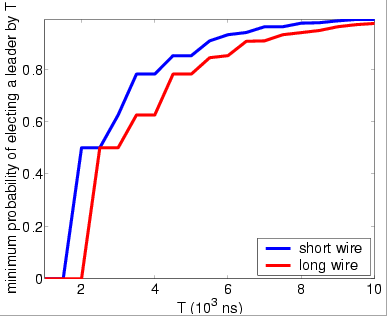
In the graph below, we have plotted the deadline probabilities for both the short and long wires.
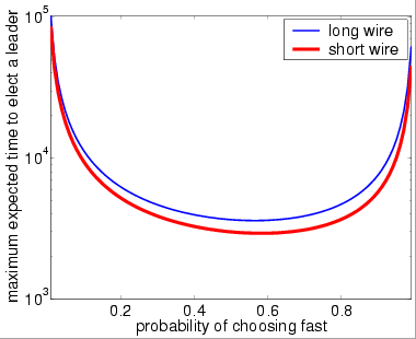
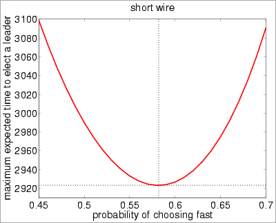
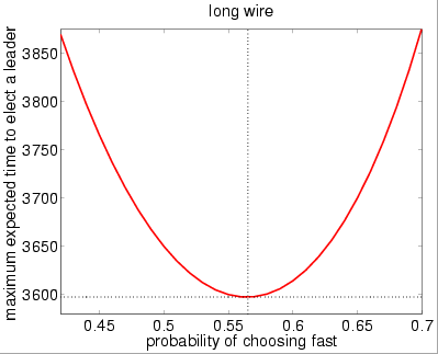
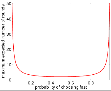
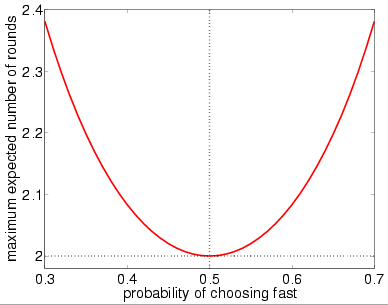
Expected reachability: for the integer semantic models we consider the effect of using a biased coin with respect to expected reachability through varying the parameter fast which equals the probability of the coin landing on 'fast' (the probability of the coin landing on 'slow' is 1-fast). The properties we consider are the maximum expected time to elect a leader and the maximum expected number of rounds until a leader is elected.
The expected time property for the model Impl is specified as follows: R{"time"}max=? [ F ( (s1=8) & (s2=7) ) | ( (s1=7) & (s2=8) ) ].
In the case of the model Abst these properties are expressed as: R{"time"}max=?[ F (s=9) ] and R{"rounds"}max=?[ F (s=9) ] respectively.Note that, all experiments were performed on the integer semantic models and the results for the expected number of rounds are the same for either of the wire lengths.
| Impl Model (short wire) | |||||
| fast: | max expected time | ||||
| iter.s: | time per iter. (s): | ||||
| 0.1 | 2,637 | 0.010 | |||
| 0.4 | 3,586 | 0.010 | |||
| 0.45 | 3,273 | 0.011 | |||
| 0.5 | 3,081 | 0.011 | |||
| 0.55 | 2,985 | 0.010 | |||
| 0.6 | 2,931 | 0.010 | |||
| 0.9 | 7,061 | 0.011 | |||
| Impl Model (long wire) | |||||
| fast: | max expected time | ||||
| iter.s: | time per iter. (s): | ||||
| 0.1 | 14,979 | 0.595 | |||
| 0.4 | 4,311 | 0.601 | |||
| 0.45 | 3,985 | 0.595 | |||
| 0.5 | 3,774 | 0.601 | |||
| 0.55 | 3,689 | 0.595 | |||
| 0.6 | 3,657 | 0.602 | |||
| 0.9 | 9,404 | 0.596 | |||
| Abst Model (short wire) | ||||||||
| fast: | max expected time | max expected rounds | ||||||
| iter.s: | time per iter. (s): | iter.s: | time per iter. (s): | |||||
| 0.1 | 6,217 | 0.0004 | 9398 | 0.0004 | ||||
| 0.4 | 2,028 | 0.0004 | 2586 | 0.0004 | ||||
| 0.45 | 1,908 | 0.0004 | 2344 | 0.0004 | ||||
| 0.5 | 1,792 | 0.0004 | 2179 | 0.0003 | ||||
| 0.55 | 1,744 | 0.0004 | 2095 | 0.0004 | ||||
| 0.6 | 1,685 | 0.0004 | 2012 | 0.0003 | ||||
| 0.9 | 3,657 | 0.0004 | 4666 | 0.0004 | ||||
| Abst Model (long wire) | ||||||||
| fast: | max expected time | max expected rounds | ||||||
| iter.s: | time per iter. (s): | iter.s: | time per iter. (s): | |||||
| 0.1 | 14,589 | 0.0008 | 10,693 | 0.0006 | ||||
| 0.4 | 4,167 | 0.0007 | 2,746 | 0.0006 | ||||
| 0.45 | 3,839 | 0.0008 | 2,501 | 0.0006 | ||||
| 0.5 | 3,633 | 0.0008 | 2,339 | 0.0006 | ||||
| 0.55 | 3,551 | 0.0007 | 2,173 | 0.0006 | ||||
| 0.6 | 3,511 | 0.0007 | 2,169 | 0.0006 | ||||
| 0.9 | 9,013 | 0.0008 | 5,301 | 0.0006 | ||||
In the graph below, we have plotted the model checking results for the expected reachability properties. Note that, the results are the same for the Abst and Impl models and the results for the maximum expected number of rounds are the same for either of the wire lengths.
