

(Muppala, Ciardo & Trivedi)
Related publications: [KNP04c, KNP07b]
This case study illustrates the applicability of probabilistic model checking and the PRISM tool to the process of dependability analysis. We model an embedded control system, closely based on the one presented in [MCT94], the structure of which is shown below.
The system comprises an input processor (I) which reads and processes data from three sensors (S1, S2, S3). It is then polled by a main processor (M) which, in turn, passes instructions to an output processor (O). This process occurs cyclically, with the length of the cycle controlled by a timer in the main processor. The output processor takes the instructions it receives and uses them to control two actuators (A1, A2). Finally, a bus connects the three processors together. A concrete example of such a system might be a gas boiler, where the sensors are thermostats and the actuators are valves.
Any of the three sensors can fail, but they are used in triple modular redundancy: the input processor can determine sufficient information to proceed provided two of the three are functional. If more than one becomes unavailable, the processor reports this fact to the main processor and the system is shut down. In similar fashion, it is sufficient for only one of the two actuators to be working, but if this is not the case, the output processor tells the main processor to shut the system down. The I/O processors themselves can also fail. This can be either a permanent fault or a transient fault. In the latter case, the situation can be rectified automatically by the processor rebooting itself. In either case, if the I or O processor is unavailable and this leads to M being unable either to read data from I or send instructions to O, then M is forced to skip the current cycle. If M detects that the number of consecutive cycles skipped exceeds a limit, MAX_COUNT, then it assumes that either I or O has failed and shuts the system down. Unless specified otherwise, we assume a value of 2 for MAX_COUNT. Lastly, the main processor can also fail, in which case the system is automatically shut down.
The mean times to failure for a sensor, actuator and processor are 1 month, 2 months and 1 year, respectively. A transient fault occurs in a processor once a day on average. The mean times for a timer cycle to expire and for a processor reboot to complete are 1 minute and 30 seconds, respectively. We assume that all these delays are distributed exponentially; hence the system can be modelled as a continuous-time Markov chain (CTMC).
Our PRISM model of the system comprises 6 modules, one for the sensors, one for the actuators, one for each processor and one for the connecting bus. Below we give the PRISM language description.
ctmc

// constants
const int MAX_COUNT;
const int MIN_SENSORS = 2;
const int MIN_ACTUATORS = 1;

// rates
const double lambda_p = 1/(365*24*60*60); // 1 year
const double lambda_s = 1/(30*24*60*60); // 1 month
const double lambda_a = 1/(2*30*24*60*60); // 2 months
const double tau = 1/60; // 1 min
const double delta_f = 1/(24*60*60); // 1 day
const double delta_r = 1/30; // 30 secs

// sensors
module sensors

	s : [0..3] init 3; // number of sensors working

	[] s>1 -> s*lambda_s : (s'=s-1); // failure of a single sensor

endmodule

// input processor
// (takes data from sensors and passes onto main processor)
module proci

	i : [0..2] init 2; // 2=ok, 1=transient fault, 0=failed

	[] i>0 & s>=MIN_SENSORS -> lambda_p : (i'=0); // failure of processor
	[] i=2 & s>=MIN_SENSORS -> delta_f : (i'=1); // transient fault
	[input_reboot] i=1 & s>=MIN_SENSORS -> delta_r : (i'=2); // reboot after transient fault

endmodule

// actuators
module actuators

	a : [0..2] init 2; // number of actuators working

	[] a>0 -> a*lambda_a : (a'=a-1); // failure of a single actuator

endmodule

// output processor
// (receives instructions from main processor and passes onto actuators)
module proco = proci [ i=o, s=a, input_reboot=output_reboot, MIN_SENSORS=MIN_ACTUATORS ] endmodule

// main processor
// (takes data from proci, processes it, and passes instructions to proco)
module procm

	m : [0..1] init 1; // 1=ok, 0=failed
	count : [0..MAX_COUNT+1] init 0; // number of consecutive skipped cycles

	// failure of processor
	[] m=1 -> lambda_p : (m'=0);
	// processing completed before timer expires - reset skipped cycle counter
	[timeout]  comp -> tau : (count'=0);
	// processing not completed before timer expires - increment skipped cycle counter
	[timeout] !comp -> tau : (count'=min(count+1, MAX_COUNT+1));

endmodule

// connecting bus
module bus

	// flags
	// main processor has processed data from input processor
	// and sent corresponding instructions to output processor (since last timeout)
	comp : bool init true;
	// input processor has data ready to send
	reqi : bool init true;
	// output processor has instructions ready to be processed
	reqo : bool init false;

	// input processor reboots
	[input_reboot]  true -> 1 :
	// performs a computation if has already done so or
	// it is up and ouput clear (i.e. nothing waiting)
	(comp'=(comp | (m=1 & !reqo)))
	// up therefore something to process
	& (reqi'=true)
	// something to process if not functioning and either
	// there is something already pending
	// or the main processor sends a request
	& (reqo'=!(o=2 & a>=1) & (reqo | m=1));

	// output processor reboots
	[output_reboot] true -> 1 :
	// performs a computation if it has already or
	// something waiting and is up
	// (can be processes as the output has come up and cleared pending requests)
	(comp'=(comp | (reqi & m=1)))
	// something to process it they are up or
	// there was already something and the main processor acts
	// (output now up must be due to main processor being down)
	& (reqi'=(i=2 & s>=2) | (reqi & m=0))
	// output and actuators up therefore nothing can be pending
	& (reqo'=false);

	// main processor times out
	[timeout] true -> 1 :
	// performs a computation if it is up something was pending
	// and nothing is waiting for the output
	(comp'=(reqi & !reqo & m=1))
	// something to process if up or
	// already something and main process cannot act
	// (down or outputs pending)
	& (reqi'=(i=2 & s>=2) | (reqi & (reqo | m=0)))
	// something to process if they are not functioning and
	// either something is already pending
	// or the main processor acts
	& (reqo'=!(o=2 & a>=1) & (reqo | (reqi & m=1)));

endmodule

// the system is down
formula down = (i=2&s<MIN_SENSORS)|(count=MAX_COUNT+1)|(o=2&a<MIN_ACTUATORS)|(m=0);
// transient failure has occured but the system is not down
formula danger = !down & (i=1 | o=1);
// the system is operational
formula up = !down & !danger;

// reward structures

rewards "up"
	up : 1/3600;
endrewards
rewards "danger"
	danger : 1/3600;
endrewards
rewards "down"
	down : 1/3600;
endrewards
The module for the sensors, includes an integer variable s representing the number of sensors currently working. The module's behaviour is described by one guarded command which represents the failure of a single sensor. Its guard "s>0" states this can occur at any time, except when all sensors have already failed. The action s'=s-1 simply decrements the counter of functioning sensors. The rate of this action is s*r, where r is the rate for a single sensor and s is the PRISM variable referred to previously which denotes the number of active sensors.
The module for the input has a single variable i with range [0..2] which indicates which of the three possible states the processor is in, i.e. whether it is working, is recovering from a transient fault, or has failed. The three guarded commands in the module correspond, respectively, to the processor failing, suffering a transient fault, and rebooting. The commands themselves are fairly self explanatory. Two points of note are as follows. Firstly, the guards of these commands can refer to variables from other modules, as evidenced by the use of s>=2. This is because the input processor ceases to function once it has detected that less than two sensors are operational. Secondly, the last command contains an additional label input_reboot, placed between the square brackets at the start of the command. This is used for synchronising actions between modules, i.e. allowing two or more modules to make transitions simultaneously. Here, this is used to notify the main processor of the reboot as soon as it occurs.
Model StatisticsThe tables below shows statistics and construction times of the models when the value of MAX_COUNT varies. The tables include:
| MAX_COUNT | States | Nodes | Leaves | Construction | ||
| Time (s) | Iter.s | |||||
| 2 | 2633 | 1194 | 9 | 0.065 | 14 | |
| 3 | 3478 | 1144 | 9 | 0.066 | 15 | |
| 4 | 4323 | 1558 | 9 | 0.082 | 16 | |
| 5 | 5168 | 1448 | 9 | 0.073 | 17 | |
| 6 | 6013 | 1586 | 9 | 0.083 | 18 | |
| 7 | 6858 | 1405 | 9 | 0.076 | 19 | |
| 8 | 7703 | 1950 | 9 | 0.082 | 20 | |
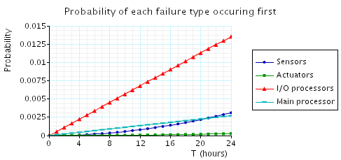
We have used PRISM to analyse a number of dependability properties using probabilistic model checking. The full list of properties is available here. First, we consider the probability of the system shutting itself down. Note that there are four distinct types of failure which can cause a shutdown: faults in
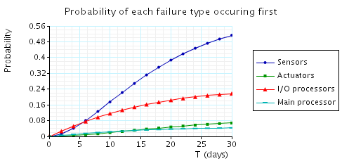
The above property denotes the probability that failure j is the first to occur. Note that, for example, if an actuator fails, the sensors, unaware of this, will continue to operate and may subsequently fail. Hence, we need to determine the likelihood of each failure occurring, before any of the others do. In the figures below, we plot the results of this computation over two ranges of values for T: the first 24 hours and the first month of operation. We can see, for example, that while initially the I/O processors are more likely to cause a system shutdown, in the long run it is the sensors which are most unreliable.
By omitting the bound <=T from the above CSL formula:
we can ask the model checker to compute the long-run failure probability of each failure type. The results are:
| Failure type | Probability | |
| Sensors | 0.6214 | |
| Actuators | 0.0877 | |
| I/O processors | 0.2425 | |
| Main processor | 0.0484 |
Note that the above probabilities sum to one, i.e. the system will eventually shut down with probability 1.
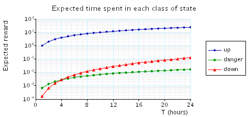
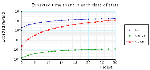
Second, we consider a number of cost-based properties. We classify the states of our model into three types: "up", where everything is functioning, "down", where the system has shut down, and "danger", where a (possibly transient) failure has occurred but has yet to cause a shutdown (e.g. if the I or O processor has failed but the M processor has yet to detect this). We can reason about the time spent in each class by assigning a cost of 1 to those states, 0 to all others (as shown in the reward structures "down", "danger" and "up" defined in the prism description above), and then computing the total cumulated reward. We use the properties:
These give us the expected time spent in each class, up until time T and before the system shuts down, respectively.
We plot the results for the first value in the figures below, again for two ranges of T: the first day and the first month of operation.
In the table below, we give the results of the second property, as we vary MAX_COUNT, the number of skipped cycles which the main processor waits before deciding that the input/output processors have failed. We see that increasing the value of MAX_COUNT increases the expected time until failure, but also has an adverse effect on the expected time spent in "danger" states.
| MAX_COUNT: | Expected time: | ||
| danger (hrs): | up (days): | ||
| 1 | 0.236 | 14.323 | |
| 2 | 0.293 | 17.660 | |
| 3 | 0.318 | 19.100 | |
| 4 | 0.327 | 19.628 | |
| 5 | 0.330 | 19.809 | |
| 6 | 0.331 | 19.871 | |
| 7 | 0.332 | 19.891 | |
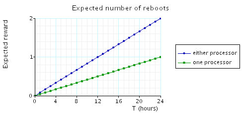
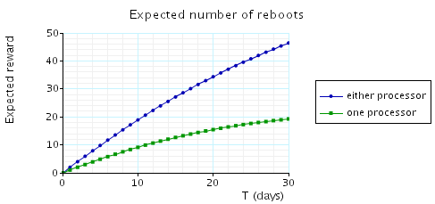
Finally, to illustrate a different type of cost structure, we compute the expected number of processor reboots which occur over time. This is done by assigning a cost of 1 to all transitions which constitute a reboot and 0 to all others. The results are plotted below.
const double T; // time bound

// causes of failues
label "fail_sensors" = i=2&s<MIN_SENSORS; // sensors have failed
label "fail_actuators" = o=2&a<MIN_ACTUATORS; // actuators have failed
label "fail_io" = count=MAX_COUNT+1; // IO has failed
label "fail_main" = m=0; // ,main processor has failed

// system status
label "down" = (i=2&s<MIN_SENSORS)|(count=MAX_COUNT+1)|(o=2&a<MIN_ACTUATORS)|(m=0); // system has shutdown
label "danger" = !down & (i=1 | o=1); // transient fault has occured
label "up" = !down & !danger; // system is operational

// Probability of any failure occurring within T hours
P=? [ true U<=T*3600 "down" ]

// Probability of each failure type occurring first (within T hours)
P=? [ !"down" U<=T*3600 "fail_sensors" ]
P=? [ !"down" U<=T*3600 "fail_actuators" ]
P=? [ !"down" U<=T*3600 "fail_io" ]
P=? [ !"down" U<=T*3600 "fail_main" ]

// Probability of each failure type occurring first (within T days)
P=? [ !"down" U<=T*3600*24 "fail_sensors" ]
P=? [ !"down" U<=T*3600*24 "fail_actuators" ]
P=? [ !"down" U<=T*3600*24 "fail_io" ]
P=? [ !"down" U<=T*3600*24 "fail_main" ]

// Probability of any failure occurring within T days
P=? [ true U<=T*3600*24 "down" ]

// Long-run probability of each failure type occurring
P=? [ !"down" U "fail_sensors" ]
P=? [ !"down" U "fail_actuators" ]
P=? [ !"down" U "fail_io" ]
P=? [ !"down" U "fail_main" ]

// Expected time spent in "up"/"danger"/"down" by time T
R{"up"}=? [ C<=T*3600 ]
R{"danger"}=? [ C<=T*3600 ]
R{"down"}=? [ C<=T*3600 ]

// Expected time spent in "up"/"danger" before "down"
R{"up"}=? [ F "down" ]
R{"danger"}=? [ F "down" ]