

(Aspnes & Herlihy)
Related publications: [KNS01a]
This case study concerns modelling and verifying the shared coin protocol of the randomised consensus algorithm of Aspnes and Herlihy [AH90] using PRISM. The shared coin protocol returns a preference 1 or 2, with a certain probability, whenever requested by a process at some point in the execution of the consensus algorithm. The shared coin protocol implements a collective random walk parameterised by the number of processes N and the constant K > 1 (independent of N). The consensus algorithm proceeds through rounds and for each round r there is a new copy of the shared coin protocol denoted CFr.
The processes access a global shared counter, initially 0. On entering the protocol, a process flips a coin, and, depending on the outcome, increments or decrements the shared counter. Since we are working in a distributed scenario, several processes may simultaneously want to flip a coin, which is modelled as a nondeterministic choice between probability distributions, one for each coin flip. Having flipped the coin, the process then reads the counter, say observing c. If c >= KN it chooses 1 as its preferred value, and if c <= -KN it chooses 2. Otherwise, the process flips the coin again, and continues doing so until it observes that the counter has passed one of the barriers.
The PRISM source code in the case when there are 8 processes is given below.
// COIN FLIPPING PROTOCOL FOR POLYNOMIAL RANDOMIZED CONSENSUS [AH90]
// gxn/dxp 20/11/00

mdp

// constants
const int N=8;
const int K;
const int range = 2*(K+1)*N;
const int counter_init = (K+1)*N;
const int left = N;
const int right = 2*(K+1)*N - N;

// shared coin
global counter : [0..range] init counter_init;

module process1

	// program counter
	pc1 : [0..3];
	// 0 - flip
	// 1 - write
	// 2 - check
	// 3 - finished

	// local coin
	coin1 : [0..1];

	// flip coin
	[] (pc1=0)  -> 0.5 : (coin1'=0) & (pc1'=1) + 0.5 : (coin1'=1) & (pc1'=1);
	// write tails -1  (reset coin to add regularity)
	[] (pc1=1) & (coin1=0) & (counter>0) -> (counter'=counter-1) & (pc1'=2) & (coin1'=0);
	// write heads +1 (reset coin to add regularity)
	[] (pc1=1) & (coin1=1) & (counter<range) -> (counter'=counter+1) & (pc1'=2) & (coin1'=0);
	// check
	// decide tails
	[] (pc1=2) & (counter<=left) -> (pc1'=3) & (coin1'=0);
	// decide heads
	[] (pc1=2) & (counter>=right) -> (pc1'=3) & (coin1'=1);
	// flip again
	[] (pc1=2) & (counter>left) & (counter<right) -> (pc1'=0);
	// loop (all loop together when done)
	[done] (pc1=3) -> (pc1'=3);

endmodule

// construct remaining processes through renaming
module process2 = process1[pc1=pc2,coin1=coin2] endmodule
module process3 = process1[pc1=pc3,coin1=coin3] endmodule
module process4 = process1[pc1=pc4,coin1=coin4] endmodule
module process5 = process1[pc1=pc5,coin1=coin5] endmodule
module process6 = process1[pc1=pc6,coin1=coin6] endmodule
module process7 = process1[pc1=pc7,coin1=coin7] endmodule
module process8 = process1[pc1=pc8,coin1=coin8] endmodule

// labels
label "finished" = pc1=3 & pc2=3 & pc3=3 & pc4=3 & pc5=3 & pc6=3 & pc7=3 & pc8=3 ;
label "all_coins_equal_0" = coin1=0 & coin2=0 & coin3=0 & coin4=0 & coin5=0 & coin6=0 & coin7=0 & coin8=0 ;
label "all_coins_equal_1" = coin1=1 & coin2=1 & coin3=1 & coin4=1 & coin5=1 & coin6=1 & coin7=1 & coin8=1 ;
label "agree" = coin1=coin2 & coin2=coin3 & coin3=coin4 & coin4=coin5 & coin5=coin6 & coin6=coin7 & coin7=coin8 ;

// rewards
rewards "steps"
	true : 1;
endrewards
The table below shows the size of the model (number of state) for various values of N and K.
| Model: | States: | ||
| N | K | ||
| 2 | 2 | 272 | |
| 4 | 528 | ||
| 8 | 1,040 | ||
| 16 | 2,064 | ||
| 32 | 4,112 | ||
| 64 | 8,208 | ||
| 4 | 2 | 22,656 | |
| 4 | 43,136 | ||
| 8 | 84,096 | ||
| 16 | 166,016 | ||
| 32 | 329,856 | ||
| 6 | 2 | 1,258,240 | |
| 4 | 2,376,448 | ||
| 8 | 4,612,864 | ||
| 16 | 9,085,696 | ||
| 8 | 2 | 61,018,112 | |
| 4 | 114,757,632 | ||
| 8 | 222,236,672 | ||
| 16 | 437,194,752 | ||
| 10 | 2 | 2,761,248,768 | |
| 4 | 5,179,854,848 | ||
| 6 | 7,598,460,928 | ||
There are two properties of the shared coin protocol we need to verify to prove Probabilistic wait free termination.
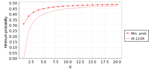
In the case of C2, we actually calculate the exact (minimum) probability of the processes drawing the same value, as opposed to a lower bound (K-1)/2K established analytically in [AH90] using random walk theory.
We express this is PRISM as follows:
P>=1 [ F "finished" ]
This is found to be satisfied in all states of the all the models listed in the table above.
In this case, we calculate the actual minimum probability, p, for which this condition holds.
For v=1, we express this is PRISM as follows:
Pmin=? [ F "finished"&"all_coins_equal_1" ]
The table below shows the computed minimum value of p and the lower bound (K-1)/2K, established analytically in [AH90] using random walk theory.
| Model: | p: | (K-1)/2K: | |||
| N | K | ||||
| 2 | 2 | 0.382814 | 0.25 | ||
| 4 | 0.437752 | 0.3125 | |||
| 8 | 0.468783 | 0.4375 | |||
| 16 | 0.484507 | 0.46875 | |||
| 32 | 0.492715 | 0.484375 | |||
| 64 | 0.498193 | 0.492188 | |||
| 4 | 2 | 0.317360 | 0.25 | ||
| 4 | 0.406307 | 0.3125 | |||
| 8 | 0.453255 | 0.4375 | |||
| 16 | 0.477088 | 0.46875 | |||
| 32 | 0.490379 | 0.484375 | |||
| 6 | 2 | 0.294365 | 0.25 | ||
| 4 | 0.395906 | 0.3125 | |||
| 8 | 0.448209 | 0.4375 | |||
| 16 | 0.475138 | 0.46875 | |||
| 8 | 2 | 0.282790 | 0.25 | ||
| 4 | 0.390749 | 0.3125 | |||
| 8 | 0.445831 | 0.4375 | |||
| 16 | 0.474747 | 0.46875 | |||
| 10 | 2 | 0.275919 | 0.25 | ||
| 4 | 0.387693 | 0.3125 | |||
| 6 | 0.425450 | 0.416667 | |||
For the case N=2, the following plot illustrates the results graphically:
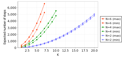
Finally, we compute the minimum and maximum expected number of steps required for completion of the algorithm.
We express this is PRISM as follows:
R{"steps"}min=? [ F "finished" ]
R{"steps"}max=? [ F "finished" ]
The results, for a selection of values of N and K are as follows:
| Model | Runtime and Problem Size Analysis for Property (1) | ||||||||
| N | K | err | States | Transitions | Runtime VI | Runtime LP | NumVars | NumCons | |
| 2 | 2 | 0.0 | 272 | 492 | 0.095 | 0.06 | 343 | 342 | |
| 2 | 0.01 | 272 | 492 | 0.087 | 0.049 | 343 | 342 | ||
| 2 | 0.05 | 272 | 492 | 0.067 | 0.05 | 343 | 342 | ||
| 2 | 0.1 | 272 | 492 | 0.088 | 0.044 | 343 | 342 | ||
| 2 | 0.15 | 272 | 492 | 0.087 | 0.05 | 343 | 342 | ||
| 4 | 0.0 | 528 | 972 | 0.474 | 0.076 | 735 | 742 | ||
| 4 | 0.01 | 528 | 972 | 0.475 | 0.095 | 735 | 742 | ||
| 4 | 0.05 | 528 | 972 | 0.483 | 0.076 | 735 | 742 | ||
| 4 | 0.1 | 528 | 972 | 0.443 | 0.076 | 735 | 742 | ||
| 4 | 0.15 | 528 | 972 | 0.427 | 0.082 | 735 | 742 | ||
| 6 | 0.0 | 784 | 1452 | 1.351 | 0.097 | 1127 | 1142 | ||
| 6 | 0.01 | 784 | 1452 | 1.31 | 0.107 | 1127 | 1142 | ||
| 6 | 0.05 | 784 | 1452 | 1.335 | 0.108 | 1127 | 1142 | ||
| 6 | 0.1 | 784 | 1452 | 1.204 | 0.098 | 1127 | 1142 | ||
| 6 | 0.15 | 784 | 1452 | 1.393 | 0.108 | 1127 | 1142 | ||
| 8 | 0.0 | 1040 | 1932 | 2.722 | 0.124 | 1519 | 1542 | ||
| 8 | 0.01 | 1040 | 1932 | 2.449 | 0.138 | 1519 | 1542 | ||
| 8 | 0.05 | 1040 | 1932 | 2.931 | 0.161 | 1519 | 1542 | ||
| 8 | 0.1 | 1040 | 1932 | 2.828 | 0.138 | 1519 | 1542 | ||
| 8 | 0.15 | 1040 | 1932 | 2.943 | 0.144 | 1519 | 1542 | ||
| 10 | 0.0 | 1296 | 2412 | 5.133 | 0.142 | 1911 | 1942 | ||
| 10 | 0.01 | 1296 | 2412 | 5.132 | 0.196 | 1911 | 1942 | ||
| 10 | 0.05 | 1296 | 2412 | 5.014 | 0.17 | 1911 | 1942 | ||
| 10 | 0.1 | 1296 | 2412 | 5.091 | 0.178 | 1911 | 1942 | ||
| 10 | 0.15 | 1296 | 2412 | 5.307 | 0.169 | 1911 | 1942 | ||