Wireless Communication Cell

(Haring, Marie, Puigjaner and Trivedi)

Contents

• Introduction
• Model Statistics
• Model Construction Times
• Model Checking

Introduction

This case study is based on a single cell in a wireless communication network. It is taken from [HMPT00]. The model includes the phenomenon of hand off which we now explain.

When a mobile station moves across a cell boundary the channel in the earlier cell is released and an idle channel is required in the target cell. If an idle channel is available in the target cell the hand off is resumed and otherwise the hand off is dropped.

Since dropping of a hand off is generally considered more serious than blocking, to reduce the probability of a hand off being dropped, a guarded channel scheme (GCS) is used: a fixed number of channels (called guarded channels) are reserved exclusively for the hand off calls.

The model is represented as a CTMC. We use N to denote the number of channels in the cell and suppose that the number of guarded channel is 20% of the total number of channels. The PRISM source code for this case study is given below.

// single cell in wireless communication network [HMPT01]
// gxn/dxp 5/3/01

ctmc

const int N; // N - number of channels
const double lambda1=49; // arrival rate of new calls
const double lambda2=21; // arrival rate of hand-off calls
const double mu=1; // departure rate of calls

module cell
	
	n : [0..N]; // number of calls in the cell
	
	// arrival of new call
	[] (n<N*0.8) -> lambda1 : (n'=n+1);
	// arrival of hand of call
	[] (n<N) -> lambda2 : (n'=n+1);
	// completion of call or mobile departs cell
	[] (n>0) -> n*mu : (n'=n-1);
	
endmodule

// rewards - number calls in the cell
rewards "calls"
	true : n;
endrewards

Extensions to this model include:

• For a fixed number of channels, vary the number of guarded channels and analyse the differences in performance.
• Consider a network of the above cells under different topologies.
• Add a control channel to a cell which is used for transmitting control messages to the system.
• Add failures and recoveries to all of the above.

Model Statistics

The table below shows statistics for each model we have built. It gives information about the CTMC representing the model: the number of states and the number of non zeros (transitions).

N:		Model:
		States:	NNZ:
50		51	100
100		101	200
150		151	300
200		201	400
250		251	500
300		301	600
350		351	700
400		401	800
450		451	900
500		501	1,000

Note that the above statistics are independent of the number of guarded channels.

Model Construction Times

The table below gives the times taken to construct the models. This process involves first building a CTMC (represented as an MTBDD) from the system description (in our module based language), and then computing the reachable states using a BDD based fixpoint algorithm. The total time required and the number of fixpoint iterations are given below.

N:		Construction:
		Time (s):	Iter.s:
50		0.058	51
100		0.093	101
150		0.128	151
200		0.139	201
250		0.188	251
300		0.269	301
350		0.245	351
400		0.296	401
450		0.345	451
500		0.425	501

Model Checking

We now report on the model checking results obtained using PRISM when verifying the following CSL properties.

const double T; // time bound

// the maximum probability that a hand off call can be dropped within t time units (assuming a guarded channel is free)
P=?[ true U<=T (n=N) {n<N}{max} ]

// the maximum probability that a call can be dropped within t time units (assuming a non-guarded channel is free)
P=?[ true U<=T (n>=N*0.8) {n<N*0.8}{max} ]

// the minimum probability that a cell will be accepted within T time units (assuming no channels are free)
P=?[ true U<=T (n<N*0.8) {n=N}{min} ]

// the expected number of calls at time T
R{"calls"}=? [ I=T ]

// the probability that in the long run any call can be dropped
S=? [ n<N*0.8 ]

// the expected number calls in the cell in the long run
R{"calls"}=? [ S ]

All experiments were carried out on a 2.0GHz PC with 512 Gb memory running Linux and in all iterative methods we stop iterating when the relative error between subsequent iteration vectors is less than 1e-6, that is:

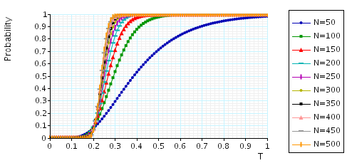
• The maximum probability that a hand off call can be dropped within t time units (assuming a guarded channel is free): the table and graph below presents the statistics and results for the model checking process.

  c:		T=0.5:
  		Iters:	Time per iter: (s)
  			MTBDD	Sparse	Hybrid
  50		227	0.000793	< 0.00001	< 0.00001
  100		247	0.002186	< 0.00001	< 0.00001
  150		268	0.000370	0.000037	0.000037
  200		288	0.000250	0.000035	0.000035
  250		309	0.000227	0.000032	0.000065
  300		335	0.000357	0.000090	0.000090
  350		360	0.000741	0.000111	0.000083
  400		386	0.000770	0.000155	0.000130
  450		411	0.000870	0.000170	0.000146
  500		437	0.000970	0.000183	0.000206

  
  

• The maximum probability that a call can be dropped within t time units (assuming a non-guarded channel is free): the graph below presents the results for this property.

  

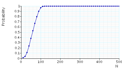
• The minimum probability that a cell will be accepted within T time units (assuming no channels are free): the graph below presents the results for this property.

  

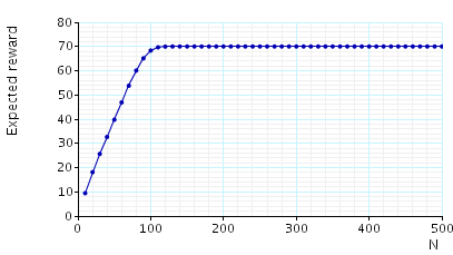
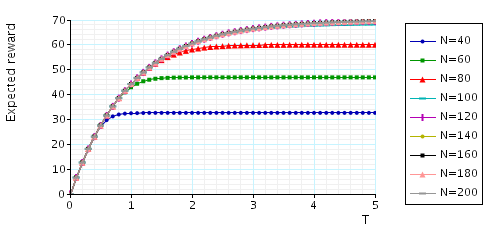
• The expected number of calls in the cell at time T: the table and graph below presents the model checking statistics for this property.

  c:		T=1:
  		Iters:	Time per iter: (s)
  			MTBDD	Sparse	Hybrid
  50		216	0.000880	< 0.00001	< 0.00001
  100		551	0.001760	0.000018	< 0.00001
  150		669	0.002661	< 0.00001	< 0.00001
  200		790	0.003557	< 0.00001	0.000013
  250		913	0.004545	0.000011	0.000011
  300		1,060	0.005519	0.000009	0.000019
  350		1,206	0.006650	0.000008	0.000017
  400		1,351	0.007646	0.000007	0.000022
  450		1,494	0.008963	0.000007	0.000027
  500		1,637	0.009505	0.000012	0.000024

  
  

• Lon run average properties: the table below gives the model checking statistics when computing the steady state probabilities for both the JOR and SOR methods when using PRISM's different engines.

  c:		JOR:					SOR:
  		Iters:	Time per iter: (s)				Iters:	Time per iter: (s)
  			MTBDD	Sparse	Hybrid			Sparse	Hybrid
  50		301	0.001018	< 0.00001	< 0.00001		173	< 0.00001	< 0.00001
  100		1,400	0.001960	< 0.00001	< 0.00001		771	< 0.00001	0.000013
  150		1,894	0.002829	0.000005	0.000011		1,139	0.000009	0.000018
  200		2,254	0.003745	0.000004	0.000009		1,298	0.000015	0.000023
  250		2,491	0.005122	0.000008	0.000012		1,419	0.000021	0.000028
  300		2,686	0.005481	0.000007	0.000011		1,520	0.000020	0.000033
  350		2,859	0.005726	0.000010	0.000017		1,611	0.000019	0.000037
  400		3,020	0.005915	0.000013	0.000017		1,696	0.000024	0.000041
  450		3,171	0.006346	0.000013	0.000019		1,776	0.000028	0.000056
  500		3,316	0.008201	0.000015	0.000021		1,854	0.000032	0.000054

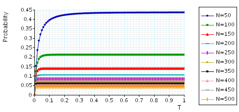
  In the graphs below we have plotted the result for the probability that in the long run any call can be dropped and the expected number of calls in the cell in the long run.

  
  

Site hosted at the Department of Computer Science, University of Oxford