
(Itai & Rodeh)
This case study is based on the synchronous leader election protocol of Itai & Rodeh [IR90]. This protocol solves the following problem.
| Given a synchronous ring of N processors design a protocol such that they will be able to elect a leader (a uniquely designated processor) by sending messages around the ring. |
The protocol proceeds in rounds and is parametrised by a constant K. Each round begins by all processors (independently) choosing a random number (uniformly) from {1,...,K} as an id. The processors then pass their ids around the ring. If there is a unique id, then the processor with the maximum unique id is elected the leader, and otherwise the processors begin a new round.
We assume that the ring is synchronous: there is a global clock and at every time slot a processor reads the message that was sent at the previous time slot (if it exists), makes at most one state transition and then may send at most one message.
By way of example, the PRISM source code for the case where N=4 and K=8 is given below.
// synchronous leader election protocol (itai & Rodeh)
// dxp/gxn 25/01/01
// N=4 and K=8

dtmc

// CONSTANTS
const N=4; // number of processes
const K=8; // range of probabilistic choice

// counter module used to count the number of processes that have been read
// and to know when a process has decided
module counter

	// counter
	c : [1..N-1];

	// reading
	[read] c<N-1 -> (c'=c+1);
	// finished reading
	[read] c=N-1 -> (c'=c);
	//done
	[done] u1 | u2 | u3 | u4 -> (c'=c);
	// pick again reset counter
	[retry] !(u1 | u2 | u3 | u4) -> (c'=1);
	// loop (when finished to avoid deadlocks)
	[loop] s1=3 -> (c'=c);

endmodule

//  processes form a ring and suppose:
// process 1 reads process 2
// process 2 reads process 3
// process 3 reads process 1
module process1

	// local state
	s1 : [0..3];
	// s1=0 make random choice
	// s1=1 reading
	// s1=2 deciding
	// s1=3 finished

	// has a unique id so far (initially true)
	u1 : bool;

	// value to be sent to next process in the ring (initially sets this to its own value)
	v1 : [0..K-1];

	// random choice
	p1 : [0..K-1];

	// pick value
	[pick] s1=0 -> 1/K : (s1'=1) & (p1'=0) & (v1'=0) & (u1'=true)
	             + 1/K : (s1'=1) & (p1'=1) & (v1'=1) & (u1'=true)
	             + 1/K : (s1'=1) & (p1'=2) & (v1'=2) & (u1'=true)
	             + 1/K : (s1'=1) & (p1'=3) & (v1'=3) & (u1'=true)
	             + 1/K : (s1'=1) & (p1'=4) & (v1'=4) & (u1'=true)
	             + 1/K : (s1'=1) & (p1'=5) & (v1'=5) & (u1'=true)
	             + 1/K : (s1'=1) & (p1'=6) & (v1'=6) & (u1'=true)
	             + 1/K : (s1'=1) & (p1'=7) & (v1'=7) & (u1'=true);
	// read
	[read] s1=1 &  u1 & !p1=v2 & c<N-1 -> (u1'=true) & (v1'=v2);
	[read] s1=1 &  u1 &  p1=v2 & c<N-1 -> (u1'=false) & (v1'=v2) & (p1'=0);
	[read] s1=1 & !u1 &  c<N-1 -> (u1'=false) & (v1'=v2);
	// read and move to decide
	[read] s1=1 &  u1 & !p1=v2 & c=N-1 -> (s1'=2) & (u1'=true) & (v1'=0) & (p1'=0);
	[read] s1=1 &  u1 &  p1=v2 & c=N-1 -> (s1'=2) & (u1'=false) & (v1'=0) & (p1'=0);
	[read] s1=1 & !u1 &  c=N-1 -> (s1'=2) & (u1'=false) & (v1'=0);
	// done
	[done] s1=2 -> (s1'=3) & (u1'=false) & (v1'=0) & (p1'=0);
	//retry
	[retry] s1=2 -> (s1'=0) & (u1'=false) & (v1'=0) & (p1'=0);
	// loop (when finished to avoid deadlocks)
	[loop] s1=3 -> (s1'=3);

endmodule

// construct remaining processes through renaming
module process2=process1[s1=s2,p1=p2,v1=v2,u1=u2,v2=v3] endmodule
module process3=process1[s1=s3,p1=p3,v1=v3,u1=u3,v2=v4] endmodule
module process4=process1[s1=s4,p1=p4,v1=v4,u1=u4,v2=v1] endmodule

// REWARDS -expected number of rounds
rewards "rounds"
	[pick] true : 1;
endrewards
The table below shows statistics for the DTMCs we have built for different values of the constants N and K. The tables include:
| N: | K: | Model: | MTBDD: | Construction: | ||||||
| States: | Transitions: | Nodes: | Leaves: | Time (s): | Iter.s: | |||||
| 3 | 2 | 22 | 29 | 367 | 3 | 0.059 | 5 | |||
| 4 | 135 | 198 | 1,781 | 3 | 0.196 | 5 | ||||
| 6 | 439 | 654 | 5,632 | 3 | 0.37 | 5 | ||||
| 8 | 1,031 | 1,542 | 10,595 | 3 | 0.658 | 5 | ||||
| 10 | 2,007 | 3,006 | 23,382 | 3 | 1.501 | 5 | ||||
| 12 | 3,466 | 5,193 | 29,617 | 3 | 1.556 | 5 | ||||
| 14 | 5,495 | 8,238 | 51,000 | 3 | 1.624 | 5 | ||||
| 16 | 8,199 | 12,294 | 69,553 | 3 | 4.719 | 5 | ||||
| 4 | 2 | 55 | 70 | 908 | 3 | 0.079 | 6 | |||
| 4 | 782 | 1,037 | 10,801 | 3 | 0.242 | 6 | ||||
| 6 | 3,902 | 5,197 | 58,324 | 3 | 1.427 | 6 | ||||
| 8 | 12,302 | 16,397 | 165,625 | 3 | 10.90 | 6 | ||||
| 10 | 30,014 | 40,013 | 473,188 | 3 | 38.38 | 6 | ||||
| 12 | 62,222 | 82,957 | 929,667 | 3 | 163.6 | 6 | ||||
| 5 | 2 | 136 | 167 | 1,731 | 3 | 0.067 | 7 | |||
| 4 | 4,124 | 5,147 | 41,528 | 3 | 0.623 | 7 | ||||
| 6 | 31,133 | 38,908 | 337,108 | 3 | 15.28 | 7 | ||||
| 8 | 131,101 | 163,868 | 1,274,313 | 3 | 231.5 | 7 | ||||
| 6 | 2 | 329 | 392 | 3,163 | 3 | 0.086 | 8 | |||
| 4 | 20,524 | 24,619 | 140,735 | 3 | 2.619 | 8 | ||||
| 6 | 233,340 | 279,995 | 1,732,096 | 3 | 561.7 | 8 | ||||
| 8 | 2 | 1803 | 2,058 | 7857 | 3 | 0.147 | 10 | |||
| 4 | 458,847 | 524,382 | 1,131,806 | 3 | 300.0 | 10 | ||||
| 10 | 2 | 9,229 | 10,252 | 16,128 | 3 | 0.276 | 12 | |||
We have model checked the following properties:
This property, in the case when N=4, can be expressed in PCTL as follows:
Model checking times:
| N: | K: | Prob1 precomputation: | ||
| Time (s): | Iterations: | |||
| 3 | 2 | 0.00 | 18 | |
| 4 | 0.01 | 18 | ||
| 6 | 0.05 | 18 | ||
| 8 | 0.09 | 18 | ||
| 10 | 0.21 | 18 | ||
| 12 | 0.35 | 18 | ||
| 14 | 0.52 | 18 | ||
| 16 | 0.74 | 18 | ||
| 4 | 2 | 0.01 | 22 | |
| 4 | 0.12 | 22 | ||
| 6 | 0.68 | 22 | ||
| 8 | 2.08 | 22 | ||
| 10 | 6.83 | 22 | ||
| 12 | 13.9 | 22 | ||
| 5 | 2 | 0.02 | 26 | |
| 4 | 0.67 | 26 | ||
| 6 | 8.33 | 26 | ||
| 8 | 116 | 26 | ||
| 6 | 2 | 0.05 | 30 | |
| 4 | 3.42 | 30 | ||
| 6 | 148 | 30 | ||
| 8 | 2 | 0.17 | 38 | |
| 4 | 72.5 | 38 | ||
| 10 | 2 | 0.43 | 46 | |
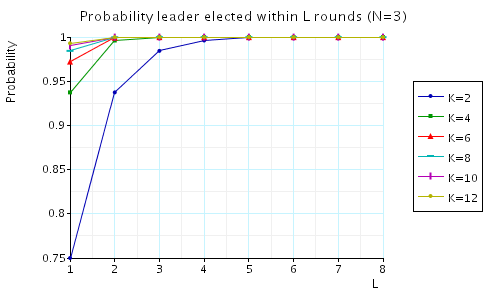
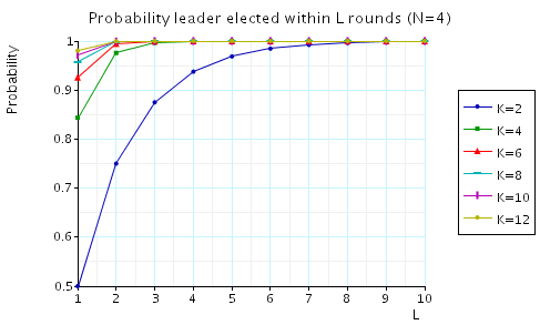
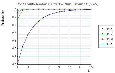
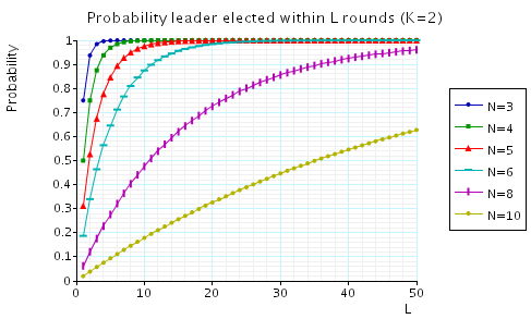
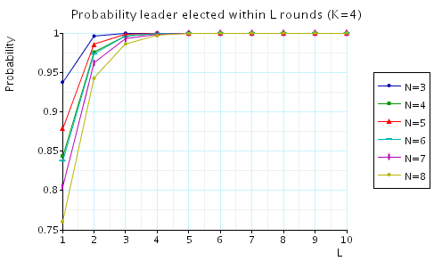
The probability of electing a leader within L rounds.
This property, in the case when N=4, can be expressed in PCTL as follows:
In the graphs below we have plotted these expected values as L varies for a range of values of N and K.
N=3
N=4
N=5
K=2
K=4
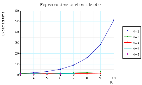
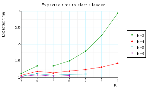
The expected number of rounds to elect a leader.
This property, in the case when N=4, can be expressed in PCTL as follows:
In the graphs below we have plotted these expected values for a range of values of N and K.