
(Ciardo & Tilgner)
This case study is based on the Kanban flexible manufacturing system of [CT96]. The model is represented as a CTMC. We use t to denote the number of tokens in the system. The PRISM source code for this case study given below.
// kanban manufacturing example [CT96]
// dxp/gxn 3/2/00

ctmc

// number of tokens
const int t;

// rates
const double in1      = 1.0;
const double out4     = 0.9;
const double synch123 = 0.4;
const double synch234 = 0.5;
const double back     = 0.3;
const double redo1    = 0.36;
const double redo2    = 0.42;
const double redo3    = 0.39;
const double redo4    = 0.33;
const double ok1      = 0.84;
const double ok2      = 0.98;
const double ok3      = 0.91;
const double ok4      = 0.77;

module k1

	w1 : [0..t];
	x1 : [0..t];
	y1 : [0..t];
	z1 : [0..t];

	[in]   (w1<t) & (x1<t) -> in1 	 : (w1'=w1+1) & (x1'=x1+1);
	[]   (x1>0) & (y1<t) -> redo1	 : (x1'=x1-1) & (y1'=y1+1);
	[]   (x1>0) & (z1<t) -> ok1 	 : (x1'=x1-1) & (z1'=z1+1);
	[]   (y1>0) & (x1<t) -> back	 : (y1'=y1-1) & (x1'=x1+1);
	[s1] (z1>0) & (w1>0) -> synch123 : (z1'=z1-1) & (w1'=w1-1);

endmodule

module k2

	w2 : [0..t];
	x2 : [0..t];
	y2 : [0..t];
	z2 : [0..t];

	[s1] (w2<t) & (x2<t) -> 1	 : (w2'=w2+1) & (x2'=x2+1);
	[]   (x2>0) & (y2<t) -> redo2 : (x2'=x2-1) & (y2'=y2+1);
	[]   (x2>0) & (z2<t) -> ok2   : (x2'=x2-1) & (z2'=z2+1);
	[]   (y2>0) & (x2<t) -> back  : (y2'=y2-1) & (x2'=x2+1);
	[s2] (z2>0) & (w2>0) -> 1	 : (z2'=z2-1) & (w2'=w2-1);

endmodule

module k3

	w3 : [0..t];
	x3 : [0..t];
	y3 : [0..t];
	z3 : [0..t];

	[s1] (w3<t) & (x3<t) -> 1	 : (w3'=w3+1) & (x3'=x3+1);
	[]   (x3>0) & (y3<t) -> redo3 : (x3'=x3-1) & (y3'=y3+1);
	[]   (x3>0) & (z3<t) -> ok3   : (x3'=x3-1) & (z3'=z3+1);
	[]   (y3>0) & (x3<t) -> back  : (y3'=y3-1) & (x3'=x3+1);
	[s2] (z3>0) & (w3>0) -> 1	 : (z3'=z3-1) & (w3'=w3-1);


endmodule

module k4

	w4 : [0..t];
	x4 : [0..t];
	y4 : [0..t];
	z4 : [0..t];

	[s2] (w4<t) & (x4<t) -> synch234 : (w4'=w4+1) & (x4'=x4+1);
	[]   (x4>0) & (y4<t) -> redo4	: (x4'=x4-1) & (y4'=y4+1);
	[]   (x4>0) & (z4<t) -> ok4  	: (x4'=x4-1) & (z4'=z4+1);
	[]   (y4>0) & (x4<t) -> back 	: (y4'=y4-1) & (x4'=x4+1);
	[]   (z4>0) & (w4>0) -> out4 	: (z4'=z4-1) & (w4'=w4-1);

endmodule

// reward structures

// tokens in cell1
rewards "tokens_cell1"
	true : x1+y1+z1;
endrewards

// tokens in cell2
rewards "tokens_cell2"
	true : x2+y2+z2;
endrewards

// tokens in cell3
rewards "tokens_cell3"
	true : x3+y3+z3;
endrewards

// tokens in cell4
rewards "tokens_cell4"
	true : x4+y4+z4;
endrewards

// throughput of the system
rewards "throughput"
	[in] true : 1;
endrewards
The table below shows statistics for each model we have built. The first section gives information about the CTMC representing the model: the number of states and the number of non zeros (transitions). The second part refers to the MTBDD which represents this CTMC: the total number of nodes, the number of leaves (terminal nodes), and the amount of memory needed to store it. The last column gives the amount of memory a sparse matrix would need to represent the same CTMC.
| t: | Model: | MTBDD: | Sparse: | ||||||
| States: | NNZ: | Nodes: | Leaves: | Kb: | Kb: | ||||
| 1 | 160 | 616 | 499 | 14 | 9.75 | 7.8 | |||
| 2 | 4,600 | 28120 | 1,685 | 14 | 32.9 | 348 | |||
| 3 | 58,400 | 446,400 | 2,474 | 14 | 48.3 | 5,459 | |||
| 4 | 454,475 | 3,979,850 | 4,900 | 14 | 95.7 | 48,414 | |||
| 5 | 2,546,432 | 24,460,016 | 6,308 | 14 | 123 | 296,588 | |||
| 6 | 11,261,376 | 115,708,992 | 7,876 | 14 | 154 | 1,399,955 | |||
| 7 | 41,644,800 | 450,455,040 | 9,521 | 14 | 186 | 5,441,445 | |||
The table below gives the times taken to construct the models. This process involves first building a CTMC (represented as an MTBDD) from the system description (in our module based language), and then computing the reachable states using a BDD based fixpoint algorithm. The total time required and the number of fixpoint iterations are given below.
| t: | Construction: | ||
| Time (s): | Iter.s: | ||
| 1 | 0.01 | 15 | |
| 2 | 0.07 | 29 | |
| 3 | 0.25 | 43 | |
| 4 | 1.28 | 57 | |
| 5 | 3.88 | 71 | |
| 6 | 6.21 | 85 | |
| 7 | 10.7 | 99 | |
We now report on the model checking results obtained using PRISM when verifying the following CSL properties.
// expected number of tokens in each cell
R{"tokens_cell1"}=? [ S ]
R{"tokens_cell2"}=? [ S ]
R{"tokens_cell3"}=? [ S ]
R{"tokens_cell4"}=? [ S ]

// expected throughput of the system
R{"throughput"}=? [ S ]
All experiments were carried out on a 2.80GHz PC with 1 Gb memory running Linux and in all iterative methods we stop iterating when the relative error between subsequent iteration vectors is less than 1e-6, that is:
The table below gives the times taken to compute the steady state probabilities using both the JOR and Gauss-Seidel methods.
The number of iterations required and the time taken using the MTBDD, sparse and hybrid engines is as follows.
| N: | Jacobi: | Gauss Seidel: | ||||||||
| Iterations: | Time per iteration: (s) | Iterations: | Time per iteration: (s) | |||||||
| MTBDD | Sparse | Hybrid | Sparse | Hybrid | ||||||
| 1 | 101 | 0.008564 | 0.000020 | 0.000020 | 200 | 0.000010 | 0.000010 | |||
| 2 | 166 | 0.574596 | 0.000199 | 0.000295 | 189 | 0.000291 | 0.000513 | |||
| 3 | 300 | 14.37466 | 0.003260 | 0.006523 | 206 | 0.004330 | 0.008534 | |||
| 4 | 466 | - | 0.029410 | 0.055227 | 323 | 0.037418 | 0.074399 | |||
| 5 | 663 | - | 0.179967 | 0.374664 | 461 | 0.222703 | 0.446436 | |||
| 6 | 891 | - | 0.898675 | 1.686580 | 622 | 1.075230 | 2.064293 | |||
| 7 | 1,148 | - | - | 6.379109 | 802 | - | 7.844989 | |||
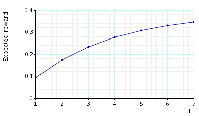
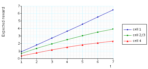
The graphs below present the results obtained for the different CSL properties.
The expected number of tokens in each cell:
The expected throughput of the system: